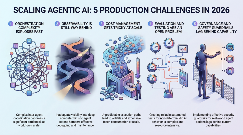
In this article, you will learn about five major challenges teams face when scaling agentic AI systems from prototype to production in 2026. Topics we will cover include: Why orchestration complexity grows rapidly in multi-agent systems. How observability, evaluation, and cost control remain difficult in production environments. Why governance and safety guardrails are becoming essential as agentic systems take real-world actions. Let’s not waste any more time. 5 Production Scaling Challenges for Agentic AI in 2026Image by Editor Introduction Everyone’s building agentic AI systems right now, for better or for worse. The demos look incredible, the prototypes feel magical, and the pitch decks practically write themselves. But here’s what nobody’s tweeting about: getting these things to actually work at scale, in production, with real users and real stakes, is a completely different game. The gap between a slick demo and a reliable production system has always existed in machine learning, but agentic AI stretches it wider than anything we’ve seen before. These systems make decisions, take actions, and chain together complex workflows autonomously. That’s powerful, and it’s also terrifying when things go sideways at scale. So let’s talk about the five biggest headaches teams are running into as they try to scale agentic AI in 2026. 1. Orchestration Complexity Explodes Fast When you’ve got a single agent handling a narrow task, orchestration feels manageable. You define a workflow, set some guardrails, and things mostly behave. But production systems rarely stay that simple. The moment you introduce multi-agent architectures in which agents delegate to other agents, retry failed steps, or dynamically choose which tools to call, you’re dealing with orchestration complexity that grows almost exponentially. Teams are finding that the coordination overhead between agents becomes the bottleneck, not the individual model calls. You’ve got agents waiting on other agents, race conditions popping up in async pipelines, and cascading failures that are genuinely hard to reproduce in staging environments. Traditional workflow engines weren’t designed for this level of dynamic decision-making, and most teams end up building custom orchestration layers that quickly become the hardest part of the entire stack to maintain. The real kicker is that these systems behave differently under load. An orchestration pattern that works beautifully at 100 requests per minute can completely fall apart at 10,000. Debugging that gap requires a kind of systems thinking that most machine learning teams are still developing. 2. Observability Is Still Way Behind You can’t fix what you can’t see, and right now, most teams can’t see nearly enough of what their agentic systems are doing in production. Traditional machine learning monitoring tracks things like latency, throughput, and model accuracy. Those metrics still matter, but they barely scratch the surface of agentic workflows. When an agent takes a 12-step journey to answer a user query, you need to understand every decision point along the way. Why did it choose Tool A over Tool B? Why did it retry step 4 three times? Why did the final output completely miss the mark, despite every intermediate step looking fine? The tracing infrastructure for this kind of deep observability is still immature. Most teams cobble together some combination of LangSmith, custom logging, and a lot of hope. What makes it harder is that agentic behavior is non-deterministic by nature. The same input can produce wildly different execution paths, which means you can’t just snapshot a failure and replay it reliably. Building robust observability for systems that are inherently unpredictable remains one of the biggest unsolved problems in the space. 3. Cost Management Gets Tricky at Scale Here’s something that catches a lot of teams off guard: agentic systems are expensive to run. Each agent action typically involves one or more LLM calls, and when agents are chaining together dozens of steps per request, the token costs add up shockingly fast. A workflow that costs $0.15 per execution sounds fine until you’re processing 500,000 requests a day. Smart teams are getting creative with cost optimization. They’re routing simpler sub-tasks to smaller, cheaper models while reserving the heavy hitters for complex reasoning steps. They’re caching intermediate results aggressively and building kill switches that terminate runaway agent loops before they burn through budget. But there’s a constant tension between cost efficiency and output quality, and finding the right balance requires ongoing experimentation. The billing unpredictability is what really stresses out engineering leads. Unlike traditional APIs, where you can estimate costs pretty accurately, agentic systems have variable execution paths that make cost forecasting genuinely difficult. One edge case can trigger a chain of retries that costs 50 times more than the normal path. 4. Evaluation and Testing Are an Open Problem How do you test a system that can take a different path every time it runs? That’s the question keeping machine learning engineers up at night. Traditional software testing assumes deterministic behavior, and traditional machine learning evaluation assumes a fixed input-output mapping. Agentic AI breaks both assumptions simultaneously. Teams are experimenting with a range of approaches. Some are building LLM-as-a-judge pipelines in which a separate model evaluates the agent’s outputs. Others are creating scenario-based test suites that check for behavioral properties rather than exact outputs. A few are investing in simulation environments where agents can be stress-tested against thousands of synthetic scenarios before hitting production. But none of these approaches feels truly mature yet. The evaluation tooling is fragmented, benchmarks are inconsistent, and there’s no industry consensus on what “good” even looks like for a complex agentic workflow. Most teams end up relying heavily on human review, which obviously doesn’t scale. 5. Governance and Safety Guardrails Lag Behind Capability Agentic AI systems can take real actions in the real world. They can send emails, modify databases, execute transactions, and interact with external services. The safety implications of that autonomy are significant, and governance frameworks haven’t kept pace with how quickly these capabilities are being deployed. The challenge is implementing guardrails that are robust enough to prevent harmful actions without being so restrictive that they kill the usefulness of

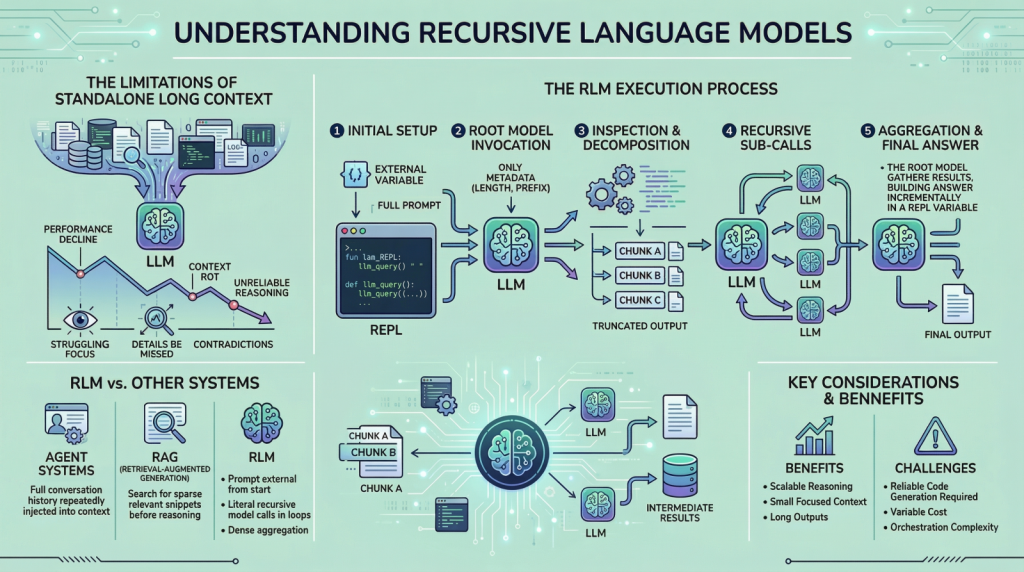
In this article, you will learn what recursive language models are, why they matter for long-input reasoning, and how they differ from standard long-context prompting, retrieval, and agentic systems. Topics we will cover include: Why long context alone does not solve reasoning over very large inputs How recursive language models use an external runtime and recursive sub-calls to process information The main tradeoffs, limitations, and practical use cases of this approach Let’s get right to it. Everything You Need to Know About Recursive Language ModelsImage by Editor Introduction If you are here, you have probably heard about recent work on recursive language models. The idea has been trending across LinkedIn and X, and it led me to study the topic more deeply and share what I learned with you. I think we can all agree that large language models (LLMs) have improved rapidly over the past few years, especially in their ability to handle large inputs. This progress has led many people to assume that long context is largely a solved problem, but it is not. If you have tried giving models very long inputs close to, or equal to, their context window, you might have noticed that they become less reliable. They often miss details present in the provided information, contradict earlier statements, or produce shallow answers instead of doing careful reasoning. This issue is often referred to as “context rot”, which is quite an interesting name. Recursive language models (RLMs) are a response to this problem. Instead of pushing more and more text into a single forward pass of a language model, RLMs change how the model interacts with long inputs in the first place. In this article, we will look at what they are, how they work, and the kinds of problems they are designed to solve. Why Long Context Is Not Enough You can skip this section if you already understand the motivation from the introduction. But if you are curious, or if the idea did not fully click the first time, let me break it down further. The way these LLMs work is fairly simple. Everything we want the model to consider is given to it as a single prompt, and based on that information, the model generates the output token by token. This works well when the prompt is short. However, when it becomes very long, performance starts to degrade. This is not necessarily due to memory limits. Even if the model can see the complete prompt, it often fails to use it effectively. Here are some reasons that may contribute to this behavior: These LLMs are mainly transformer-based models with an attention mechanism. As the prompt grows longer, attention becomes more diffuse. The model struggles to focus sharply on what matters when it has to attend to tens or hundreds of thousands of tokens. Another reason is the presence of heterogeneous information mixed together, such as logs, documents, code, chat history, and intermediate outputs. Lastly, many tasks are not just about retrieving or finding a relevant snippet in a huge body of content. They often involve aggregating information across the entire input. Because of the problems discussed above, people proposed ideas such as summarization and retrieval. These approaches do help in some cases, but they are not universal solutions. Summaries are lossy by design, and retrieval assumes that relevance can be identified reliably before reasoning begins. Many real-world tasks violate these assumptions. This is why RLMs suggest a different approach. Instead of forcing the model to absorb the entire prompt at once, they let the model actively explore and process the prompt. Now that we have the basic background, let us look more closely at how this works. How a Recursive Language Model Works in Practice In an RLM setup, the prompt is treated as part of the external environment. This means the model does not read the entire input directly. Instead, the input sits outside the model, often as a variable, and the model is given only metadata about the prompt along with instructions on how to access it. When the model needs information, it issues commands to examine specific parts of the prompt. This simple design keeps the model’s internal context small and focused, even when the underlying input is extremely large. To understand RLMs more concretely, let us walk through a typical execution step by step. Step 1: Initializing a Persistent REPL Environment At the beginning of an RLM run, the system initializes a runtime environment, typically a Python REPL. This environment contains: A variable holding the full user prompt, which may be arbitrarily large A function (for example, llm_query(…) or sub_RLM(…)) that allows the system to invoke additional language model calls on selected pieces of text From the user’s perspective, the interface remains simple, with a textual input and an output, but internally the REPL acts as scaffolding that enables scalable reasoning. Step 2: Invoking the Root Model with Prompt Metadata Only The root language model is then invoked, but it does not receive the full prompt. Instead, it is given: Constant-size metadata about the prompt, such as its length or a short prefix Instructions describing the task Access instructions for interacting with the prompt via the REPL environment By withholding the full prompt, the system forces the model to interact with the input intentionally, rather than passively absorbing it into the context window. From this point onward, the model interacts with the prompt indirectly. Step 3: Inspecting and Decomposing the Prompt via Code Execution The model might begin by inspecting the structure of the input. For example, it can print the first few lines, search for headings, or split the text into chunks based on delimiters. These operations are performed by generating code, which is then executed in the environment. The outputs of these operations are truncated before being shown to the model, ensuring that the context window is not overwhelmed. Step 4: Issuing Recursive Sub-Calls on Selected Slices Once the model understands the structure of the

In this article, you will learn how to extract seven useful readability and text-complexity features from raw text using the Textstat Python library. Topics we will cover include: How Textstat can quantify readability and text complexity for downstream machine learning tasks. How to compute seven commonly used readability metrics in Python. How to interpret these metrics when using them as features for classification or regression models. Let’s not waste any more time. 7 Readability Features for Your Next Machine Learning ModelImage by Editor Introduction Unlike fully structured tabular data, preparing text data for machine learning models typically entails tasks like tokenization, embeddings, or sentiment analysis. While these are undoubtedly useful features, the structural complexity of text — or its readability, for that matter — can also constitute an incredibly informative feature for predictive tasks such as classification or regression. Textstat, as its name suggests, is a lightweight and intuitive Python library that can help you obtain statistics from raw text. Through readability scores, it provides input features for models that can help distinguish between a casual social media post, a children’s fairy tale, or a philosophy manuscript, to name a few. This article introduces seven insightful examples of text analysis that can be easily conducted using the Textstat library. Before we get started, make sure you have Textstat installed: While the analyses described here can be scaled up to a large text corpus, we will illustrate them with a toy dataset consisting of a small number of labeled texts. Bear in mind, however, that for downstream machine learning model training and inference, you will need a sufficiently large dataset for training purposes. import pandas as pd import textstat # Create a toy dataset with three markedly different texts data = { ‘Category’: [‘Simple’, ‘Standard’, ‘Complex’], ‘Text’: [ “The cat sat on the mat. It was a sunny day. The dog played outside.”, “Machine learning algorithms build a model based on sample data, known as training data, to make predictions.”, “The thermodynamic properties of the system dictate the spontaneous progression of the chemical reaction, contingent upon the activation energy threshold.” ] } df = pd.DataFrame(data) print(“Environment set up and dataset ready!”) import pandas as pd import textstat   # Create a toy dataset with three markedly different texts data = {     ‘Category’: [‘Simple’, ‘Standard’, ‘Complex’],     ‘Text’: [         “The cat sat on the mat. It was a sunny day. The dog played outside.”,         “Machine learning algorithms build a model based on sample data, known as training data, to make predictions.”,         “The thermodynamic properties of the system dictate the spontaneous progression of the chemical reaction, contingent upon the activation energy threshold.”     ] }   df = pd.DataFrame(data) print(“Environment set up and dataset ready!”) 1. Applying the Flesch Reading Ease Formula The first text analysis metric we will explore is the Flesch Reading Ease formula, one of the earliest and most widely used metrics for quantifying text readability. It evaluates a text based on the average sentence length and the average number of syllables per word. While it is conceptually meant to take values in the 0 – 100 range — with 0 meaning unreadable and 100 meaning very easy to read — its formula is not strictly bounded, as shown in the examples below: df[‘Flesch_Ease’] = df[‘Text’].apply(textstat.flesch_reading_ease) print(“Flesch Reading Ease Scores:”) print(df[[‘Category’, ‘Flesch_Ease’]]) df[‘Flesch_Ease’] = df[‘Text’].apply(textstat.flesch_reading_ease)   print(“Flesch Reading Ease Scores:”) print(df[[‘Category’, ‘Flesch_Ease’]]) Output: Flesch Reading Ease Scores: Category Flesch_Ease 0 Simple 105.880000 1 Standard 45.262353 2 Complex -8.045000 Flesch Reading Ease Scores:    Category  Flesch_Ease 0    Simple   105.880000 1  Standard    45.262353 2   Complex    –8.045000 This is what the actual formula looks like: $$ 206.835 – 1.015 \left( \frac{\text{total words}}{\text{total sentences}} \right) – 84.6 \left( \frac{\text{total syllables}}{\text{total words}} \right) $$ Unbounded formulas like Flesch Reading Ease can hinder the proper training of a machine learning model, which is something to take into consideration during later feature engineering tasks. 2. Computing Flesch-Kincaid Grade Levels Unlike the Reading Ease score, which provides a single readability value, the Flesch-Kincaid Grade Level assesses text complexity using a scale similar to US school grade levels. In this case, higher values indicate greater complexity. Be warned, though: this metric also behaves similarly to the Flesch Reading Ease score, such that extremely simple or complex texts can yield scores below zero or arbitrarily high values, respectively. df[‘Flesch_Grade’] = df[‘Text’].apply(textstat.flesch_kincaid_grade) print(“Flesch-Kincaid Grade Levels:”) print(df[[‘Category’, ‘Flesch_Grade’]]) df[‘Flesch_Grade’] = df[‘Text’].apply(textstat.flesch_kincaid_grade)   print(“Flesch-Kincaid Grade Levels:”) print(df[[‘Category’, ‘Flesch_Grade’]]) Output: Flesch-Kincaid Grade Levels: Category Flesch_Grade 0 Simple -0.266667 1 Standard 11.169412 2 Complex 19.350000 Flesch–Kincaid Grade Levels:    Category  Flesch_Grade 0    Simple     –0.266667 1  Standard     11.169412 2   Complex     19.350000 3. Computing the SMOG Index Another measure with origins in assessing text complexity is the SMOG Index, which estimates the years of formal education required to comprehend a text. This formula is somewhat more bounded than others, as it has a strict mathematical floor slightly above 3. The simplest of our three example texts falls at the absolute minimum for this measure in terms of complexity. It takes into account factors such as the number of polysyllabic words, that is, words with three or more syllables. df[‘SMOG_Index’] = df[‘Text’].apply(textstat.smog_index) print(“SMOG Index Scores:”) print(df[[‘Category’, ‘SMOG_Index’]]) df[‘SMOG_Index’] = df[‘Text’].apply(textstat.smog_index)   print(“SMOG Index Scores:”) print(df[[‘Category’, ‘SMOG_Index’]]) Output: SMOG Index Scores: Category SMOG_Index 0 Simple 3.129100 1 Standard 11.208143 2 Complex 20.267339 SMOG Index Scores:    Category  SMOG_Index 0    Simple    3.129100 1  Standard   11.208143 2   Complex   20.267339 4. Calculating the Gunning Fog Index Like the SMOG Index, the Gunning Fog Index also has a strict floor, in this case equal to zero. The reason is straightforward: it quantifies the percentage of complex words along with average sentence length. It is a popular metric for analyzing business texts and ensuring that technical or domain-specific content is accessible to a wider audience. df[‘Gunning_Fog’] = df[‘Text’].apply(textstat.gunning_fog) print(“Gunning Fog Index:”) print(df[[‘Category’, ‘Gunning_Fog’]]) df[‘Gunning_Fog’] = df[‘Text’].apply(textstat.gunning_fog)   print(“Gunning Fog Index:”) print(df[[‘Category’, ‘Gunning_Fog’]]) Output: Gunning Fog Index: Category Gunning_Fog 0 Simple 2.000000 1 Standard 11.505882 2 Complex 26.000000 Gunning Fog Index:    Category  Gunning_Fog 0    Simple     2.000000 1  Standard    11.505882 2   Complex    26.000000 5. Calculating the Automated

In this article, you will learn practical strategies for building useful machine learning solutions when you have limited compute, imperfect data, and little to no engineering support. Topics we will cover include: What “low-resource” really looks like in practice. Why lightweight models and simple workflows often outperform complexity in constrained settings. How to handle messy and missing data, plus simple transfer learning tricks that still work with small datasets. Let’s get started. Building Smart Machine Learning in Low-Resource SettingsImage by Author Most people who want to build machine learning models do not have powerful servers, pristine data, or a full-stack team of engineers. Especially if you live in a rural area and run a small business (or you are just starting out with minimal tools), you probably do not have access to many resources. But you can still build powerful, useful solutions. Many meaningful machine learning projects happen in places where computing power is limited, the internet is unreliable, and the “dataset” looks more like a shoebox full of handwritten notes than a Kaggle competition. But that’s also where some of the most clever ideas come to life. Here, we will talk about how to make machine learning work in those environments, with lessons pulled from real-world projects, including some smart patterns seen on platforms like StrataScratch. What Low-Resource Really Means In summary, working in a low-resource setting likely looks like this: Outdated or slow computers Patchy or no internet Incomplete or messy data A one-person “data team” (probably you) These constraints might feel limiting, but there is still a lot of potential for your solutions to be smart, efficient, and even innovative. Why Lightweight Machine Learning Is Actually a Power Move The truth is that deep learning gets a lot of hype, but in low-resource environments, lightweight models are your best friend. Logistic regression, decision trees, and random forests may sound old-school, but they get the job done. They’re fast. They’re interpretable. And they run beautifully on basic hardware. Plus, when you’re building tools for farmers, shopkeepers, or community workers, clarity matters. People need to trust your models, and simple models are easier to explain and understand. Common wins with classic models: Crop classification Predicting stock levels Equipment maintenance forecasting So, don’t chase complexity. Prioritize clarity. Turning Messy Data into Magic: Feature Engineering 101 If your dataset is a little (or a lot) chaotic, welcome to the club. Broken sensors, missing sales logs, handwritten notes… we’ve all been there. Here’s how you can extract meaning from messy inputs: 1. Temporal Features Even inconsistent timestamps can be useful. Break them down into: Day of week Time since last event Seasonal flags Rolling averages 2. Categorical Grouping Too many categories? You can group them. Instead of tracking every product name, try “perishables,” “snacks,” or “tools.” 3. Domain-Based Ratios Ratios often beat raw numbers. You can try: Fertilizer per acre Sales per inventory unit Water per plant 4. Robust Aggregations Use medians instead of means to handle wild outliers (like sensor errors or data-entry typos). 5. Flag Variables Flags are your secret weapon. Add columns like: “Manually corrected data” “Sensor low battery” “Estimate instead of actual” They give your model context that matters. Missing Data? Missing data can be a problem, but it is not always. It can be information in disguise. It’s important to handle it with care and clarity. Treat Missingness as a Signal Sometimes, what’s not filled in tells a story. If farmers skip certain entries, it might indicate something about their situation or priorities. Stick to Simple Imputation Go with medians, modes, or forward-fill. Fancy multi-model imputation? Skip it if your laptop is already wheezing. Use Domain Knowledge Field experts often have smart rules, like using average rainfall during planting season or known holiday sales dips. Avoid Complex Chains Don’t try to impute everything from everything else; it just adds noise. Define a few solid rules and stick to them. Small Data? Meet Transfer Learning Here’s a cool trick: you don’t need massive datasets to benefit from the big leagues. Even simple forms of transfer learning can go a long way. Text Embeddings Got inspection notes or written feedback? Use small, pretrained embeddings. Big gains with low cost. Global to Local Take a global weather-yield model and adjust it using a few local samples. Linear tweaks can do wonders. Feature Selection from Benchmarks Use public datasets to guide what features to include, especially if your local data is noisy or sparse. Time Series Forecasting Borrow seasonal patterns or lag structures from global trends and customize them for your local needs. A Real-World Case: Smarter Crop Choices in Low-Resource Farming A useful illustration of lightweight machine learning comes from a StrataScratch project that works with real agricultural data from India. The goal of this project is to recommend crops that match the actual conditions farmers are working with: messy weather patterns, imperfect soil, all of it. The dataset behind it is modest: about 2,200 rows. But it covers important details like soil nutrients (nitrogen, phosphorus, potassium) and pH levels, plus basic climate information like temperature, humidity, and rainfall. Here is a sample of the data: Instead of reaching for deep learning or other heavy methods, the analysis stays intentionally simple. We start with some descriptive statistics: df.select_dtypes(include=[‘int64’, ‘float64’]).describe() df.select_dtypes(include=[‘int64’, ‘float64’]).describe() Then, we proceed to some visual exploration: # Setting the aesthetic style of the plots sns.set_theme(style=”whitegrid”) # Creating visualizations for Temperature, Humidity, and Rainfall fig, axes = plt.subplots(1, 3, figsize=(14, 5)) # Temperature Distribution sns.histplot(df[‘temperature’], kde=True, color=”skyblue”, ax=axes[0]) axes[0].set_title(‘Temperature Distribution’) # Humidity Distribution sns.histplot(df[‘humidity’], kde=True, color=”olive”, ax=axes[1]) axes[1].set_title(‘Humidity Distribution’) # Rainfall Distribution sns.histplot(df[‘rainfall’], kde=True, color=”gold”, ax=axes[2]) axes[2].set_title(‘Rainfall Distribution’) plt.tight_layout() plt.show() 1 2 3 4 5 6 7 8 9 10 11 12 13 14 15 16 17 18 19 20 # Setting the aesthetic style of the plots sns.set_theme(style=“whitegrid”)   # Creating visualizations for Temperature, Humidity, and Rainfall fig, axes = plt.subplots(1, 3, figsize=(14, 5))   # Temperature Distribution sns.histplot(df[‘temperature’], kde=True, color=“skyblue”, ax=axes[0])

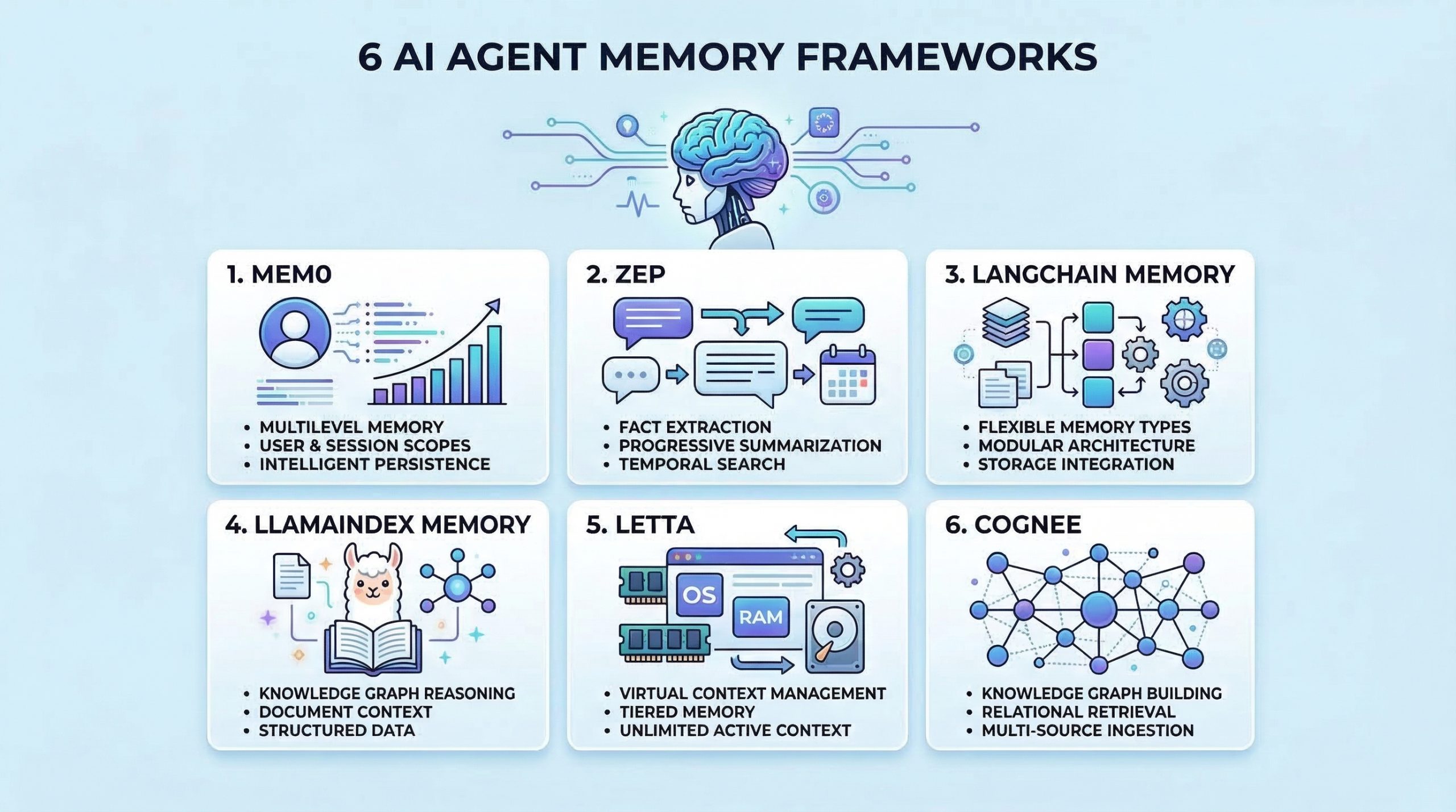
In this article, you will learn six practical frameworks you can use to give AI agents persistent memory for better context, recall, and personalization. Topics we will cover include: What “agent memory” means and why it matters for real-world assistants. Six frameworks for long-term memory, retrieval, and context management. Practical project ideas to get hands-on experience with agent memory. Let’s get right to it. The 6 Best AI Agent Memory Frameworks You Should Try in 2026Image by Editor Introduction Memory helps AI agents evolve from stateless tools into intelligent assistants that learn and adapt. Without memory, agents cannot learn from past interactions, maintain context across sessions, or build knowledge over time. Implementing effective memory systems is also complex because you need to handle storage, retrieval, summarization, and context management. As an AI engineer building agents, you need frameworks that go beyond simple conversation history. The right memory framework enables your agents to remember facts, recall past experiences, learn user preferences, and retrieve relevant context when needed. In this article, we’ll explore AI agent memory frameworks that are useful for: Storing and retrieving conversation history Managing long-term factual knowledge Implementing semantic memory search Handling context windows effectively Personalizing agent behavior based on past interactions Let’s explore each framework. ⚠️ Note: This article is not an exhaustive list, but rather an overview of top frameworks in the space, presented in no particular ranked order. 1. Mem0 Mem0 is a dedicated memory layer for AI applications that provides intelligent, personalized memory capabilities. It is designed specifically to give agents long-term memory that persists across sessions and evolves over time. Here’s why Mem0 stands out for agent memory: Extracts and stores relevant facts from conversations Provides multi-level memory supporting user-level, session-level, and agent-level memory scopes Uses vector search combined with metadata filtering for hybrid memory retrieval that is both semantic and precise Includes built-in memory management features and version control for memories Start with the Quickstart Guide to Mem0, then explore Memory Types and Memory Filters in Mem0. 2. Zep Zep is a long-term memory store designed specifically for conversational AI applications. It focuses on extracting facts, summarizing conversations, and providing relevant context to agents efficiently. What makes Zep excellent for conversational memory: Extracts entities, intents, and facts from conversations and stores them in a structured format Provides progressive summarization that condenses long conversation histories while preserving key information Offers both semantic and temporal search, allowing agents to find memories based on meaning or time Supports session management with automatic context building, providing agents with relevant memories for each interaction Start with the Quick Start Guide and then refer to the Zep Cookbook page for practical examples. 3. LangChain Memory LangChain includes a comprehensive memory module that provides various memory types and strategies for different use cases. It’s highly flexible and integrates seamlessly with the broader LangChain ecosystem. Here’s why LangChain Memory is valuable for agent applications: Offers multiple memory types including conversation buffer, summary, entity, and knowledge graph memory for different scenarios Supports memory backed by various storage options, from simple in-memory stores to vector databases and traditional databases Provides memory classes that can be easily swapped and combined to create hybrid memory systems Integrates natively with chains, agents, and other LangChain components for consistent memory handling Memory overview – Docs by LangChain has everything you need to get started. 4. LlamaIndex Memory LlamaIndex provides memory capabilities integrated with its data framework. This makes it particularly strong for agents that need to remember and reason over structured information and documents. What makes LlamaIndex Memory useful for knowledge-intensive agents: Combines chat history with document context, allowing agents to remember both conversations and referenced information Provides composable memory modules that work seamlessly with LlamaIndex’s query engines and data structures Supports memory with vector stores, enabling semantic search over past conversations and retrieved documents Handles context window management, condensing or retrieving relevant history as needed Memory in LlamaIndex is a comprehensive overview of short and long-term memory in LlamaIndex. 5. Letta Letta takes inspiration from operating systems to manage LLM context, implementing a virtual context management system that intelligently moves information between immediate context and long-term storage. It’s one of the most unique approaches to solving the memory problem for AI agents. What makes Letta work great for context management: Uses a tiered memory architecture mimicking OS memory hierarchy, with main context as RAM and external storage as disk Allows agents to control their memory through function calls for reading, writing, and archiving information Handles context window limitations by intelligently swapping information in and out of the active context Enables agents to maintain effectively unlimited memory despite fixed context window constraints, making it ideal for long-running conversational agents Intro to Letta is a good starting point. You can then look at Core Concepts and LLMs as Operating Systems: Agent Memory by DeepLearning.AI. 6. Cognee Cognee is an open-source memory and knowledge graph layer for AI applications that structures, connects, and retrieves information with precision. It is designed to give agents a dynamic, queryable understanding of data — not just stored text, but interconnected knowledge. Here’s why Cognee stands out for agent memory: Builds knowledge graphs from unstructured data, enabling agents to reason over relationships rather than only retrieve isolated facts Supports multi-source ingestion including documents, conversations, and external data, unifying memory across diverse inputs Combines graph traversal with vector search for retrieval that understands how concepts relate, not just how similar they are Includes pipelines for continuous memory updates, letting knowledge evolve as new information flows in Start with the Quickstart Guide and then move to Setup Configuration to get started. Wrapping Up The frameworks covered here provide different approaches to solving the memory challenge. To gain practical experience with agent memory, consider building some of these projects: Create a personal assistant with Mem0 that learns your preferences and recalls past conversations across sessions Build a customer service agent with Zep that remembers customer history and provides personalized support Develop a research agent with LangChain

In this article, you will learn how to use a pre-trained large language model to extract structured features from text and combine them with numeric columns to train a supervised classifier. Topics we will cover include: Creating a toy dataset with mixed text and numeric fields for classification Using a Groq-hosted LLaMA model to extract JSON features from ticket text with a Pydantic schema Training and evaluating a scikit-learn classifier on the engineered tabular dataset Let’s not waste any more time. From Text to Tables: Feature Engineering with LLMs for Tabular DataImage by Editor Introduction While large language models (LLMs) are typically used for conversational purposes in use cases that revolve around natural language interactions, they can also assist with tasks like feature engineering on complex datasets. Specifically, you can leverage pre-trained LLMs from providers like Groq (for example, models from the Llama family) to undertake data transformation and preprocessing tasks, including turning unstructured data like text into fully structured, tabular data that can be used to fuel predictive machine learning models. In this article, I will guide you through the full process of applying feature engineering to structured text, turning it into tabular data suitable for a machine learning model — namely, a classifier trained on features created from text by using an LLM. Setup and Imports First, we will make all the necessary imports for this practical example: import pandas as pd import json from pydantic import BaseModel, Field from openai import OpenAI from google.colab import userdata from sklearn.ensemble import RandomForestClassifier from sklearn.model_selection import train_test_split from sklearn.metrics import classification_report from sklearn.preprocessing import StandardScaler import pandas as pd import json from pydantic import BaseModel, Field from openai import OpenAI from google.colab import userdata from sklearn.ensemble import RandomForestClassifier from sklearn.model_selection import train_test_split from sklearn.metrics import classification_report from sklearn.preprocessing import StandardScaler Note that besides common libraries for machine learning and data preprocessing like scikit-learn, we import the OpenAI class — not because we will directly use an OpenAI model, but because many LLM APIs (including Groq’s) have adopted the same interface style and specifications as OpenAI. This class therefore helps you interact with a variety of providers and access a wide range of LLMs through a single client, including Llama models via Groq, as we will see shortly. Next, we set up a Groq client to enable access to a pre-trained LLM that we can call via API for inference during execution: groq_api_key = userdata.get(‘GROQ_API_KEY’) client = OpenAI( base_url=”https://api.groq.com/openai/v1″, api_key=groq_api_key ) groq_api_key = userdata.get(‘GROQ_API_KEY’) client = OpenAI(     base_url=“https://api.groq.com/openai/v1”,     api_key=groq_api_key ) Important note: for the above code to work, you need to define an API secret key for Groq. In Google Colab, you can do this through the “Secrets” icon on the left-hand side bar (this icon looks like a key). Here, give your key the name ‘GROQ_API_KEY’, then register on the Groq website to get an actual key, and paste it into the value field. Creating a Toy Ticket Dataset The next step generates a synthetic, partly random toy dataset for illustrative purposes. If you have your own text dataset, feel free to adapt the code accordingly and use your own. import random import time random.seed(42) categories = [“access”, “inquiry”, “software”, “billing”, “hardware”] templates = { “access”: [ “I’ve been locked out of my account for {days} days and need urgent help!”, “I can’t log in, it keeps saying bad password.”, “Reset my access credentials immediately.”, “My 2FA isn’t working, please help me get into my account.” ], “inquiry”: [ “When will my new credit card arrive in the mail?”, “Just checking on the status of my recent order.”, “What are your business hours on weekends?”, “Can I upgrade my current plan to the premium tier?” ], “software”: [ “The app keeps crashing every time I try to view my transaction history.”, “Software bug: the submit button is greyed out.”, “Pages are loading incredibly slowly since the last update.”, “I’m getting a 500 Internal Server Error on the dashboard.” ], “billing”: [ “I need a refund for the extra charges on my bill.”, “Why was I billed twice this month?”, “Please update my payment method, the old card expired.”, “I didn’t authorize this $49.99 transaction.” ], “hardware”: [ “My hardware token is broken, I can’t log in.”, “The screen on my physical device is cracked.”, “The card reader isn’t scanning properly anymore.”, “Battery drains in 10 minutes, I need a replacement unit.” ] } data = [] for _ in range(100): cat = random.choice(categories) # Injecting a random number of days into specific templates to foster variety text = random.choice(templates[cat]).format(days=random.randint(1, 14)) data.append({ “text”: text, “account_age_days”: random.randint(1, 2000), “prior_tickets”: random.choices([0, 1, 2, 3, 4, 5], weights=[40, 30, 15, 10, 3, 2])[0], “label”: cat }) df = pd.DataFrame(data) 1 2 3 4 5 6 7 8 9 10 11 12 13 14 15 16 17 18 19 20 21 22 23 24 25 26 27 28 29 30 31 32 33 34 35 36 37 38 39 40 41 42 43 44 45 46 47 48 49 50 51 52 53 import random import time   random.seed(42) categories = [“access”, “inquiry”, “software”, “billing”, “hardware”]   templates = {     “access”: [         “I’ve been locked out of my account for {days} days and need urgent help!”,         “I can’t log in, it keeps saying bad password.”,         “Reset my access credentials immediately.”,         “My 2FA isn’t working, please help me get into my account.”     ],     “inquiry”: [         “When will my new credit card arrive in the mail?”,         “Just checking on the status of my recent order.”,         “What are your business hours on weekends?”,         “Can I upgrade my current plan to the premium tier?”     ],     “software”: [         “The app keeps crashing every time I try to view my transaction history.”,         “Software bug: the submit button is greyed out.”,         “Pages are loading incredibly slowly since the last update.”,         “I’m getting a 500 Internal Server Error on the dashboard.”     ],     “billing”: [         “I need a refund for the extra charges on my bill.”,         “Why

In this article, you will learn how to use Google Colab’s AI-assisted coding features — especially AI prompt cells — to generate, explain, and refine Python code directly in the notebook environment. Topics we will cover include: How AI prompt cells work in Colab and where to find them A practical workflow for generating code and running it safely in executable code cells Key limitations to keep in mind and when to use the “magic wand” Gemini panel instead Let’s get on with it. Setting Up a Google Colab AI-Assisted Coding Environment That Actually WorksImage by Editor Introduction This article focuses on Google Colab, an increasingly popular, free, and accessible, cloud-based Python environment that is well-suited for prototyping data analysis workflows and experimental code before moving to production systems. Based on the latest freely available version of Google Colab at the time of writing, we adopt a step-by-step tutorial style to explore how to make effective use of its recently introduced AI-assisted coding features. Yes: Colab now incorporates tools for AI-assisted coding, such as code generation from natural language, explanations of written code, auto-completion, and smart troubleshooting. Looking into Colab’s AI-Assisted Capabilities First, we sign in to Google Colab with a Google account of our choice and click “New Notebook” to start a fresh coding workspace. The good news: all of this is done in the cloud, and all you need is a web browser (ideally Chrome); nothing needs to be installed locally. Here is the big novelty: if you are familiar with Colab, you would be familiar with its two basic types of cells: code cells, for writing and executing code; and text cells, to supplement your code with descriptions, explanations, and even embedded visuals to explain what is going on in your code. Now, there is a third type of cell, and it is not clearly identifiable at first glance: its name is the AI prompt cell. This is a brand-new, special cell type that supports direct, one-shot interaction with Google’s most powerful generative AI models from the Gemini family, and it is especially helpful for those with limited coding knowledge. Creating an AI prompt cell is simple: in the upper toolbar, right below the menus, click on the little dropdown arrow next to “Code” and select “Add AI prompt cell”. Something like this should appear in your still blank notebook. Creating an AI prompt cell to generate code from natural language Let’s give it a try by writing the following in the “Ask me anything…” textbox: Write Python code that generates 100 values for five different types of weather forecast values, and plots a histogram of these values Be patient for a few seconds, even if it seems like nothing happens at first. The AI is working on your request behind the scenes. Eventually, you may get a response from the selected Gemini model that looks like this: Taking advantage of AI prompt cells and executable code cells This new feature provides a comfortable AI-assisted coding environment that is ideal not only for code generation, but also for quick prototyping, exploring new ideas, or even making existing code more self-explanatory, e.g. by prompting the AI to insert explainable features or informative print statements in relevant parts of a program. Understanding the capabilities of this new cell type is key to leveraging Colab’s newest AI-assisted coding features correctly. A standard code cell right below each of your AI prompt cells makes for a practical symbiosis. Why? Because the output of AI prompt cells is not directly executable code, since it often comes with text descriptions before and/or after the code. Simply copy the code portion of the response and paste it into a code cell below to try it. Not everything works as expected? No problem. The AI prompt cell stays there, in its dedicated place in your notebook, so you can continue the interaction and refine your code until it fully meets your requirements. Be aware, however, of some limitations of this newly introduced cell type. Regardless of where in your notebook an AI prompt cell is located, it is not automatically aware of the content in the rest of your notebook. You will need to provide your code to an AI prompt cell in order to ask something about it. For instance, imagine we placed the previously generated code in several code cells for step-by-step execution. Then, at the bottom of the notebook, we add another AI prompt cell and ask the following: AI response when asking for code outside the AI prompt cell Notice the response: the AI is asking you to explicitly provide (paste) the code you want it to analyze, explain, and so on, no matter where that code exists in the notebook. You also cannot reference cells by identifiers like #7 or #16, nor ask something like “rewrite the third code cell in a more concise, Pythonic style“. Here is a summary of the best-practice workflow we recommend getting used to: Add AI prompt cells immediately after a cell (or small group of cells) where you expect a lot of analysis, refining, and potential changes in the code. Paste the target code and use explicit instructions with action verbs like “explain”, “refactor”, “simplify”, “add error handling”, and so on. Review and execute the results manually in a backup code cell, carefully placed depending on your data transformation workflow (it may need to go before or after the cell containing the original code). AI prompt cells are great for comfortable code-creation experimentation in the main playground, but bear in mind that for other AI-assisted tasks like explaining a piece of code in a cell or transforming it, the magic wand icon available in a code cell — which opens a Gemini tab on the right-hand side of Colab for continued interaction — is still the best and most flexible approach. Wrapping Up Google Colab is continuously releasing new AI-assisted coding features, with clear strengths but also important limitations. In this article, we

Deploying AI Agents to Production: Architecture, Infrastructure, and Implementation Roadmap – MachineLearningMastery.com Deploying AI Agents to Production: Architecture, Infrastructure, and Implementation Roadmap – MachineLearningMastery.com

In this article, you will learn how vector databases and graph RAG differ as memory architectures for AI agents, and when each approach is the better fit. Topics we will cover include: How vector databases store and retrieve semantically similar unstructured information. How graph RAG represents entities and relationships for precise, multi-hop retrieval. How to choose between these approaches, or combine them in a hybrid agent-memory architecture. With that in mind, let’s get straight to it. Vector Databases vs. Graph RAG for Agent Memory: When to Use WhichImage by Author Introduction AI agents need long-term memory to be genuinely useful in complex, multi-step workflows. An agent without memory is essentially a stateless function that resets its context with every interaction. As we move toward autonomous systems that manage persistent tasks (such as like coding assistants that track project architecture or research agents that compile ongoing literature reviews) the question of how to store, retrieve, and update context becomes critical. Currently, the industry standard for this task is the vector database, which uses dense embeddings for semantic search. Yet, as the need for more complex reasoning grows, graph RAG, an architecture that combines knowledge graphs with large language models (LLMs), is gaining traction as a structured memory architecture. At a glance, vector databases are ideal for broad similarity matching and unstructured data retrieval, while graph RAG excels when context windows are limited and when multi-hop relationships, factual accuracy, and complex hierarchical structures are required. This distinction highlights vector databases’ focus on flexible matching, compared with graph RAG’s ability to reason through explicit relationships and preserve accuracy under tighter constraints. To clarify their respective roles, this article explores the underlying theory, practical strengths, and limitations of both approaches for agent memory. In doing so, it provides a practical framework to guide the choice of system, or combination of systems, to deploy. Vector Databases: The Foundation of Semantic Agent Memory Vector databases represent memory as dense mathematical vectors, or embeddings, situated in high-dimensional space. An embedding model maps text, images, or other data to arrays of floats, where the geometric distance between two vectors corresponds to their semantic similarity. AI agents primarily use this approach to store unstructured text. A common use case is storing conversational history, allowing the agent to recall what a user previously asked by searching its memory bank for semantically related past interactions. Agents also leverage vector stores to retrieve relevant documents, API documentation, or code snippets based on the implicit meaning of a user’s prompt, which is a far more robust approach than relying on exact keyword matches. Vector databases are strong choices for agent memory. They offer fast search, even across billions of vectors. Developers also find them easier to set up than structured databases. To integrate a vector store, you split the text, generate embeddings, and index the results. These databases also handle fuzzy matching well, accommodating typos and paraphrasing without requiring strict queries. But semantic search has limits for advanced agent memory. Vector databases often cannot follow multi-step logic. For instance, if an agent needs to find the link between entity A and entity C but only has data showing that A connects to B and B connects to C, a simple similarity search may miss important information. These databases also struggle when retrieving large amounts of text or dealing with noisy results. With dense, interconnected facts (from software dependencies to company organizational charts) they can return related but irrelevant information. This can crowd the agent’s context window with less useful data. Graph RAG: Structured Context and Relational Memory Graph RAG addresses the limitations of semantic search by combining knowledge graphs with LLMs. In this paradigm, memory is structured as discrete entities represented as nodes (for example, a person, a company, or a technology), and the explicit relationships between them are represented as edges (for example, “works at” or “uses”). Agents using graph RAG create and update a structured world model. As they gather new information, they extract entities and relationships and add them to the graph. When searching memory, they follow explicit paths to retrieve the exact context. The main strength of graph RAG is its precision. Because retrieval follows explicit relationships rather than semantic closeness alone, the risk of error is lower. If a relationship does not exist in the graph, the agent cannot infer it from the graph alone. Graph RAG excels at complex reasoning and is ideal for answering structured questions. To find the direct reports of a manager who approved a budget, you trace a path through the organization and approval chain — a simple graph traversal, but a difficult task for vector search. Explainability is another major advantage. The retrieval path is a clear, auditable sequence of nodes and edges, not an opaque similarity score. This matters for enterprise applications that require compliance and transparency. On the downside, graph RAG introduces significant implementation complexity. It demands robust entity-extraction pipelines to parse raw text into nodes and edges, which often requires carefully tuned prompts, rules, or specialized models. Developers must also design and maintain an ontology or schema, which can be rigid and difficult to evolve as new domains are encountered. The cold-start problem is also prominent: unlike a vector database, which is useful the moment you embed text, a knowledge graph requires substantial upfront effort to populate before it can answer complex queries. The Comparison Framework: When to Use Which When architecting memory for an AI agent, keep in mind that vector databases excel at handling unstructured, high-dimensional data and are well suited to similarity search, whereas graph RAG is advantageous for representing entities and explicit relationships when those relationships are crucial. The choice should be driven by the data’s inherent structure and the expected query patterns. Vector databases are ideally suited to purely unstructured data — chat logs, general documentation, or sprawling knowledge bases built from raw text. They excel when the query intent is to explore broad themes, such as “Find me concepts similar to X”

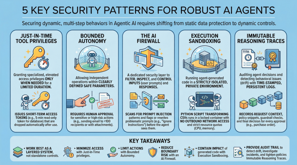
5 Essential Security Patterns for Robust Agentic AIImage by Editor Introduction Agentic AI, which revolves around autonomous software entities called agents, has reshaped the AI landscape and influenced many of its most visible developments and trends in recent years, including applications built on generative and language models. With any major technology wave like agentic AI comes the need to secure these systems. Doing so requires a shift from static data protection to safeguarding dynamic, multi-step behaviors. This article lists 5 key security patterns for robust AI agents and highlights why they matter. 1. Just-in-Time Tool Privileges Often abbreviated as JIT, this is a security model that grants users or applications specialized or elevated access privileges only when needed, and only for a limited period of time. It stands in contrast to classic, permanent privileges that remain in place unless manually modified or revoked. In the realm of agentic AI, an example would be issuing short term access tokens to limits the “blast radius” if the agent becomes compromised. Example: Before an agent runs a billing reconciliation job, it requests a narrowly scoped, 5-minute read-only token for a single database table and automatically drops the token as soon as the query completes. 2. Bounded Autonomy This security principle allows AI agents to operate independently within a bounded setting, meaning within clearly defined safe parameters, striking a balance between control and efficiency. This is especially important in high-risk scenarios where catastrophic errors from full autonomy can be avoided by requiring human approval for sensitive actions. In practice, this creates a control plane to reduce risk and support compliance requirements. Example: An agent may draft and schedule outbound emails on its own, but any message to more than 100 recipients (or containing attachments) is routed to a human for approval before sending. 3. The AI Firewall This refers to a dedicated security layer that filters, inspects, and controls inputs (user prompts) and subsequent responses to safeguard AI systems. It helps protect against threats such as prompt injection, data exfiltration, and toxic or policy-violating content. Example: Incoming prompts are scanned for prompt-injection patterns (for example, requests to ignore prior instructions or to reveal secrets), and flagged prompts are either blocked or rewritten into a safer form before the agent sees them. 4. Execution Sandboxing Take a strictly isolated, private environment or network perimeter and run any agent-generated code within it: this is known as execution sandboxing. It helps prevent unauthorized access, resource exhaustion, and potential data breaches by containing the impact of untrusted or unpredictable execution. Example: An agent that writes a Python script to transform CSV files runs it inside a locked-down container with no outbound network access, strict CPU/memory quotas, and a read-only mount of the input data. 5. Immutable Reasoning Traces This practice supports auditing autonomous agent decisions and detecting behavioral issues such as drift. It entails building time-stamped, tamper-evident, and persistent logs that capture the agent’s inputs, key intermediate artifacts used for decision-making, and policy checks. This is a crucial step toward transparency and accountability for autonomous systems, particularly in high-stakes application domains like procurement and finance. Example: For every purchase order the agent approves, it records the request context, the retrieved policy snippets, the applied guardrail checks, and the final decision in a write-once log that can be independently verified during audits. Key Takeaways These patterns work best as a layered system rather than standalone controls. Just-in-time tool privileges minimize what an agent can access at any moment, while bounded autonomy limits which actions it can take without oversight. The AI firewall reduces risk at the interaction boundary by filtering and shaping inputs and outputs, and execution sandboxing contains the impact of any code the agent generates or executes. Finally, immutable reasoning traces provide the audit trail that lets you detect drift, investigate incidents, and continuously tighten policies over time. Security Pattern Description Just-in-Time Tool Privileges Grant short-lived, narrowly scoped access only when needed to reduce the blast radius of compromise. Bounded Autonomy Constrain which actions an agent can take independently, routing sensitive steps through approvals and guardrails. The AI Firewall Filter and inspect prompts and responses to block or neutralize threats like prompt injection, data exfiltration, and toxic content. Execution Sandboxing Run agent-generated code in an isolated environment with strict resource and access controls to contain harm. Immutable Reasoning Traces Create time-stamped, tamper-evident logs of inputs, intermediate artifacts, and policy checks for auditability and drift detection. Together, these limitations reduce the chance of a single failure turning into a systemic breach, without eliminating the operational benefits that make agentic AI appealing.