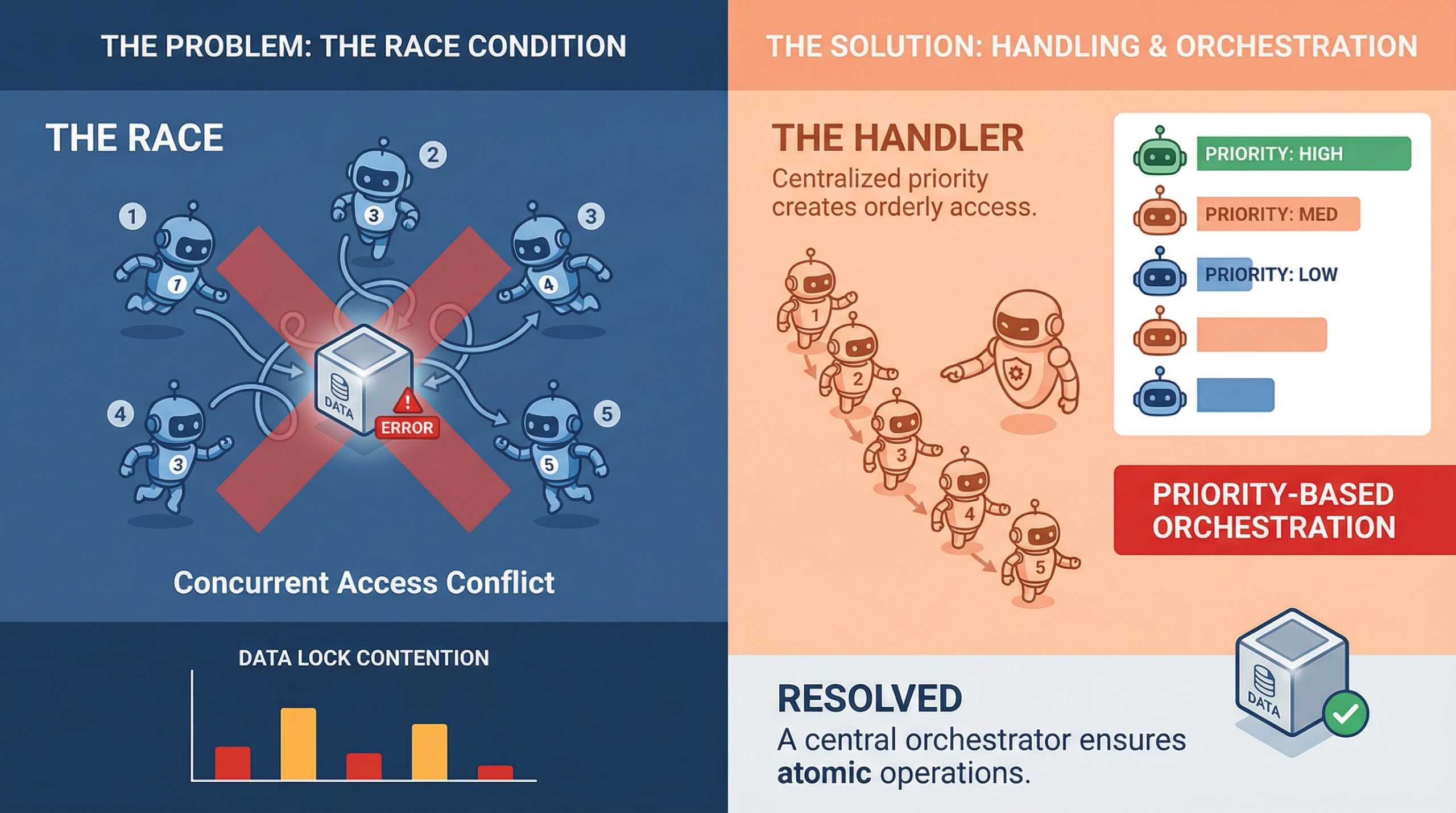
In this article, you will learn how to identify, understand, and mitigate race conditions in multi-agent orchestration systems. Topics we will cover include: What race conditions look like in multi-agent environments Architectural patterns for preventing shared-state conflicts Practical strategies like idempotency, locking, and concurrency testing Let’s get straight to it. Handling Race Conditions in Multi-Agent OrchestrationImage by Editor If you’ve ever watched two agents confidently write to the same resource at the same time and produce something that makes zero sense, you already know what a race condition feels like in practice. It’s one of those bugs that doesn’t show up in unit tests, behaves perfectly in staging, and then detonates in production during your highest-traffic window. In multi-agent systems, where parallel execution is the whole point, race conditions aren’t edge cases. They’re expected guests. Understanding how to handle them is less about being defensive and more about building systems that assume chaos by default. What Race Conditions Actually Look Like in Multi-Agent Systems A race condition happens when two or more agents try to read, modify, or write shared state at the same time, and the final result depends on which one gets there first. In a single-agent pipeline, that’s manageable. In a system with five agents running concurrently, it’s a genuinely different problem. The tricky part is that race conditions aren’t always obvious crashes. Sometimes they’re silent. Agent A reads a document, Agent B updates it half a second later, and Agent A writes back a stale version with no error thrown anywhere. The system looks fine. The data is compromised. What makes this worse in machine learning pipelines specifically is that agents often work on mutable shared objects, whether that’s a shared memory store, a vector database, a tool output cache, or a simple task queue. Any of these can become a contention point when multiple agents start pulling from them simultaneously. Why Multi-Agent Pipelines Are Especially Vulnerable Traditional concurrent programming has decades of tooling around race conditions: threads, mutexes, semaphores, and atomic operations. Multi-agent large language model (LLM) systems are newer, and they are often built on top of async frameworks, message brokers, and orchestration layers that don’t always give you fine-grained control over execution order. There’s also the problem of non-determinism. LLM agents don’t always take the same amount of time to complete a task. One agent might finish in 200ms, while another takes 2 seconds, and the orchestrator has to handle that gracefully. When it doesn’t, agents start stepping on each other, and you end up with a corrupted state or conflicting writes that the system silently accepts. Agent communication patterns matter a lot here, too. If agents are sharing state through a central object or a shared database row rather than passing messages, they are almost guaranteed to run into write conflicts at scale. This is as much a design pattern issue as it is a concurrency issue, and fixing it usually starts at the architecture level before you even touch the code. Locking, Queuing, and Event-Driven Design The most direct way to handle shared resource contention is through locking. Optimistic locking works well when conflicts are rare: each agent reads a version tag alongside the data, and if the version has changed by the time it tries to write, the write fails and retries. Pessimistic locking is more aggressive and reserves the resource before reading. Both approaches have trade-offs, and which one fits depends on how often your agents are actually colliding. Queuing is another solid approach, especially for task assignment. Instead of multiple agents polling a shared task list directly, you push tasks into a queue and let agents consume them one at a time. Systems like Redis Streams, RabbitMQ, or even a basic Postgres advisory lock can handle this well. The queue becomes your serialization point, which takes the race out of the equation for that particular access pattern. Event-driven architectures go further. Rather than agents reading from shared state, they react to events. Agent A completes its work and emits an event. Agent B listens for that event and picks up from there. This creates looser coupling and naturally reduces the overlap window where two agents might be modifying the same thing at once. Idempotency Is Your Best Friend Even with solid locking and queuing in place, things still go wrong. Networks hiccup, timeouts happen, and agents retry failed operations. If those retries are not idempotent, you will end up with duplicate writes, double-processed tasks, or compounding errors that are painful to debug after the fact. Idempotency means that running the same operation multiple times produces the same result as running it once. For agents, that often means including a unique operation ID with every write. If the operation has already been applied, the system recognizes the ID and skips the duplicate. It’s a small design choice with a significant impact on reliability. It’s worth building idempotency in from the start at the agent level. Retrofitting it later is painful. Agents that write to databases, update records, or trigger downstream workflows should all carry some form of deduplication logic, because it makes the whole system more resilient to the messiness of real-world execution. Testing for Race Conditions Before They Test You The hard part about race conditions is reproducing them. They are timing-dependent, which means they often only appear under load or in specific execution sequences that are difficult to reproduce in a controlled test environment. One useful approach is stress testing with intentional concurrency. Spin up multiple agents against a shared resource simultaneously and observe what breaks. Tools like Locust, pytest-asyncio with concurrent tasks, or even a simple ThreadPoolExecutor can help simulate the kind of overlapping execution that exposes contention bugs in staging rather than production. Property-based testing is underused in this context. If you can define invariants that should always hold regardless of execution order, you can run randomized tests that attempt to violate them. It won’t catch everything, but it will surface many of the

In the previous article, we saw how a language model converts logits into probabilities and samples the next token. But where do these logits come from? In this tutorial, we take a hands-on approach to understand the generation pipeline: How the prefill phase processes your entire prompt in a single parallel pass How the decode phase generates tokens one at a time using previously computed context How the KV cache eliminates redundant computation to make decoding efficient By the end, you will understand the two-phase mechanics behind LLM inference and why the KV cache is essential for generating long responses at scale. Let’s get started. From Prompt to Prediction: Understanding Prefill, Decode, and the KV Cache in LLMsPhoto by Neda Astani. Some rights reserved. Overview This article is divided into three parts; they are: How Attention Works During Prefill The Decode Phase of LLM Inference KV Cache: How to Make Decode More Efficient How Attention Works During Prefill Consider the prompt: Today’s weather is so … As humans, we can infer the next token should be an adjective, because the last word “so” is a setup. We also know it probably describes weather, so words like “nice” or “warm” are more likely than something unrelated like “delicious“. Transformers arrive at the same conclusion through attention. During prefill, the model processes the entire prompt in a single forward pass. Every token attends to itself and all tokens before it, building up a contextual representation that captures relationships across the full sequence. The mechanism behind this is the scaled dot-product attention formula: $$\text{Attention}(Q, K, V) = \mathrm{softmax}\left(\frac{QK^\top}{\sqrt{d_k}}\right)V$$ We will walk through this concretely below. To make the attention computation traceable, we assign each token a scalar value representing the information it carries: Position Tokens Values 1 Today 10 2 weather 20 3 is 1 4 so 5 Words like “is” and “so” carry less semantic weight than “Today” or “weather“, and as we’ll see, attention naturally reflects this. Attention Heads In real transformers, attention weights are continuous values learned during training through the $Q$ and $K$ dot product. The behavior of attention heads are learned and usually impossible to describe. No head is hardwired to “attend to even positions”. The four rules below are simplified illustration to make attention mechanism more intuitive, while the weighted aggregation over $V$ is the same. Here are the rules in our toy example: Attend to tokens at even number positions Attend to the last token Attend to the first token Attend to every token For simplicity in this example, the outputs from these heads are then combined (averaged). Let’s walk through the prefill process: Today Even tokens → none Last token → Today → 10 First token → Today → 10 All tokens → Today → 10 weather Even tokens → weather → 20 Last token → weather → 20 First token → Today → 10 All tokens → average(Today, weather) → 15 is Even tokens → weather → 20 Last token → is → 1 First token → Today → 10 All tokens → average(Today, weather, is) → 10.33 so Even tokens → average(weather, so) → 12.5 Last token → so → 5 First token → Today → 10 All tokens → average(Today, weather, is, so) → 9 Parallelizing Attention If the prompt contained 100,000 tokens, computing attention step-by-step would be extremely slow. Fortunately, attention can be expressed as tensor operations, allowing all positions to be computed in parallel. This is the key idea of prefill phase in LLM inference: When you provide a prompt, there are multiple tokens in it and they can be processed in parallel. Such parallel processing helps speed up the response time for the first token generated. To prevent tokens from seeing future tokens, we apply a causal mask, so they can only attend to itself and earlier tokens. import torch tokens = [“Today”, “weather”, “is”, “so”] n = len(tokens) d_k = 64 V = torch.tensor([[10.], [20.], [1.], [5.]], dtype=torch.float32) positions = torch.arange(1, n + 1).float() # 1-based: [1, 2, 3, 4] idx = torch.arange(n) causal_mask = idx.unsqueeze(1) >= idx.unsqueeze(0) print(causal_mask) import torch   tokens = [“Today”, “weather”, “is”, “so”] n = len(tokens) d_k = 64   V = torch.tensor([[10.], [20.], [1.], [5.]], dtype=torch.float32) positions = torch.arange(1, n + 1).float() # 1-based: [1, 2, 3, 4] idx = torch.arange(n)   causal_mask = idx.unsqueeze(1) >= idx.unsqueeze(0) print(causal_mask) Output: tensor([[ True, False, False, False], [ True, True, False, False], [ True, True, True, False], [ True, True, True, True]]) tensor([[ True, False, False, False],         [ True, True, False, False],         [ True, True, True, False],         [ True, True, True, True]]) Now, we can start writing the “rules” for the 4 attention heads. Rather than computing scores from learned $Q$ and $K$ vectors, we handcraft them directly to match our four attention rules. Each head produces a score matrix of shape (n, n), with one score per query-key pair, which gets masked and passed through softmax to produce attention weights: def selector(condition, size): “””Return a (size, d_k) tensor of +1/-1 depending on condition.””” val = torch.where(condition, torch.ones( size), -torch.ones(size)) # (size,) # (size, d_k) return val.unsqueeze(1).expand(size, d_k).contiguous() # Shared query: every row asks for a property, and K encodes which tokens match it. Q = torch.ones(n, d_k) # Head 1: select even positions # K says whether each token is at an even position. K1 = selector(positions % 2 == 0, n) scores1 = (Q @ K1.T) / (d_k ** 0.5) # Head 2: select the last token # K says whether each token is the last one. K2 = selector(positions == n, n) scores2 = (Q @ K2.T) / (d_k ** 0.5) # Head 3: select the first token # K says whether each token is the first one. K3 = selector(positions == 1, n) scores3 = (Q @ K3.T) / (d_k ** 0.5) # Head 4: select all visible tokens uniformly # K says all the tokens K4 = selector(positions == positions, n) scores4

In this article, you will learn how to implement state-managed interruptions in LangGraph so an agent workflow can pause for human approval before resuming execution. Topics we will cover include: What state-managed interruptions are and why they matter in agentic AI systems. How to define a simple LangGraph workflow with a shared agent state and executable nodes. How to pause execution, update the saved state with human approval, and resume the workflow. Read on for all the info. Building a ‘Human-in-the-Loop’ Approval Gate for Autonomous AgentsImage by Editor Introduction In agentic AI systems, when an agent’s execution pipeline is intentionally halted, we have what is known as a state-managed interruption. Just like a saved video game, the “state” of a paused agent — its active variables, context, memory, and planned actions — is persistently saved, with the agent placed in a sleep or waiting state until an external trigger resumes its execution. The significance of state-managed interruptions has grown alongside progress in highly autonomous, agent-based AI applications for several reasons. Not only do they act as effective safety guardrails to recover from otherwise irreversible actions in high-stakes settings, but they also enable human-in-the-loop approval and correction. A human supervisor can reconfigure the state of a paused agent and prevent undesired consequences before actions are carried out based on an incorrect response. LangGraph, an open-source library for building stateful large language model (LLM) applications, supports agent-based workflows with human-in-the-loop mechanisms and state-managed interruptions, thereby improving robustness against errors. This article brings all of these elements together and shows, step by step, how to implement state-managed interruptions using LangGraph in Python under a human-in-the-loop approach. While most of the example processes defined below are meant to be automated by an agent, we will also show how to make the workflow stop at a key point where human review is needed before execution resumes. Step-by-Step Guide First, we pip install langgraph and make the necessary imports for this practical example: from typing import TypedDict from langgraph.graph import StateGraph, END from langgraph.checkpoint.memory import MemorySaver from typing import TypedDict from langgraph.graph import StateGraph, END from langgraph.checkpoint.memory import MemorySaver Notice that one of the imported classes is named StateGraph. LangGraph uses state graphs to model cyclic, complex workflows that involve agents. There are states representing the system’s shared memory (a.k.a. the data payload) and nodes representing actions that define the execution logic used to update this state. Both states and nodes need to be explicitly defined and checkpointed. Let’s do that now. class AgentState(TypedDict): draft: str approved: bool sent: bool class AgentState(TypedDict):     draft: str     approved: bool     sent: bool The agent state is structured similarly to a Python dictionary because it inherits from TypedDict. The state acts like our “save file” as it is passed between nodes. Regarding nodes, we will define two of them, each representing an action: drafting an email and sending it. def draft_node(state: AgentState): print(“[Agent]: Drafting the email…”) # The agent builds a draft and updates the state return {“draft”: “Hello! Your server update is ready to be deployed.”, “approved”: False, “sent”: False} def send_node(state: AgentState): print(f”[Agent]: Waking back up! Checking approval status…”) if state.get(“approved”): print(“[System]: SENDING EMAIL ->”, state[“draft”]) return {“sent”: True} else: print(“[System]: Draft was rejected. Email aborted.”) return {“sent”: False} def draft_node(state: AgentState):     print(“[Agent]: Drafting the email…”)     # The agent builds a draft and updates the state     return {“draft”: “Hello! Your server update is ready to be deployed.”, “approved”: False, “sent”: False}   def send_node(state: AgentState):     print(f“[Agent]: Waking back up! Checking approval status…”)     if state.get(“approved”):         print(“[System]: SENDING EMAIL ->”, state[“draft”])         return {“sent”: True}     else:         print(“[System]: Draft was rejected. Email aborted.”)         return {“sent”: False} The draft_node() function simulates an agent action that drafts an email. To make the agent perform a real action, you would replace the print() statements that simulate the behavior with actual instructions that execute it. The key detail to notice here is the object returned by the function: a dictionary whose fields match those in the agent state class we defined earlier. Meanwhile, the send_node() function simulates the action of sending the email. But there is a catch: the core logic for the human-in-the-loop mechanism lives here, specifically in the check on the approved status. Only if the approved field has been set to True — by a human, as we will see, or by a simulated human intervention — is the email actually sent. Once again, the actions are simulated through simple print() statements for the sake of simplicity, keeping the focus on the state-managed interruption mechanism. What else do we need? An agent workflow is described by a graph with multiple connected states. Let’s define a simple, linear sequence of actions as follows: workflow = StateGraph(AgentState) # Adding action nodes workflow.add_node(“draft_message”, draft_node) workflow.add_node(“send_message”, send_node) # Connecting nodes through edges: Start -> Draft -> Send -> End workflow.set_entry_point(“draft_message”) workflow.add_edge(“draft_message”, “send_message”) workflow.add_edge(“send_message”, END) workflow = StateGraph(AgentState)   # Adding action nodes workflow.add_node(“draft_message”, draft_node) workflow.add_node(“send_message”, send_node)   # Connecting nodes through edges: Start -> Draft -> Send -> End workflow.set_entry_point(“draft_message”) workflow.add_edge(“draft_message”, “send_message”) workflow.add_edge(“send_message”, END) To implement the database-like mechanism that saves the agent state, and to introduce the state-managed interruption when the agent is about to send a message, we use this code: # MemorySaver is like our “database” for saving states memory = MemorySaver() # THIS IS A KEY PART OF OUR PROGRAM: telling the agent to pause before sending app = workflow.compile( checkpointer=memory, interrupt_before=[“send_message”] ) # MemorySaver is like our “database” for saving states memory = MemorySaver()   # THIS IS A KEY PART OF OUR PROGRAM: telling the agent to pause before sending app = workflow.compile(     checkpointer=memory,     interrupt_before=[“send_message”] ) Now comes the real action. We will execute the action graph defined a few moments ago. Notice below that a thread ID is used so the memory can keep track of the workflow state across executions. config = {“configurable”: {“thread_id”: “demo-thread-1”}} initial_state = {“draft”: “”, “approved”: False, “sent”: False} print(“\n— RUNNING INITIAL GRAPH —“) # The graph will run

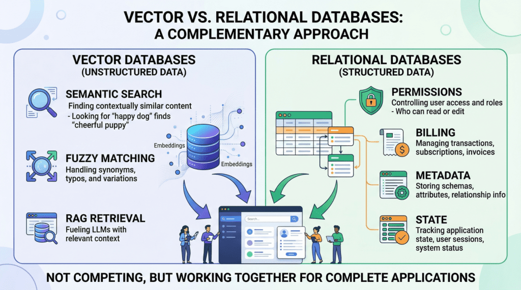
In this article, you will learn why production AI applications need both a vector database for semantic retrieval and a relational database for structured, transactional workloads. Topics we will cover include: What vector databases do well, and where they fall short in production AI systems. Why relational databases remain essential for permissions, metadata, billing, and application state. How hybrid architectures, including the use of pgvector, combine both approaches into a practical data layer. Keep reading for all the details. Beyond the Vector Store: Building the Full Data Layer for AI ApplicationsImage by Author Introduction If you look at the architecture diagram of almost any AI startup today, you will see a large language model (LLM) connected to a vector store. Vector databases have become so closely associated with modern AI that it is easy to treat them as the entire data layer, the one database you need to power a generative AI product. But once you move beyond a proof-of-concept chatbot and start building something that handles real users, real permissions, and real money, a vector database alone is not enough. Production AI applications need two complementary data engines working in lockstep: a vector database for semantic retrieval, and a relational database for everything else. This is not a controversial claim once you examine what each system actually does — though it is often overlooked. Vector databases like Pinecone, Milvus, or Weaviate excel at finding data based on meaning and intent, using high-dimensional embeddings to perform rapid semantic search. Relational databases like PostgreSQL or MySQL manage structured data with SQL, providing deterministic queries, complex filtering, and strict ACID guarantees that vector stores lack by design. They serve entirely different functions, and a robust AI application depends on both. In this article, we will explore the specific strengths and limitations of each database type in the context of AI applications, then walk through practical hybrid architectures that combine them into a unified, production-grade data layer. Vector Databases: What They Do Well and Where They Break Down Vector databases power the retrieval step in retrieval augmented generation (RAG), the pattern that lets you feed specific, proprietary context to a language model to reduce hallucinations. When a user queries your AI agent, the application embeds that query into a high-dimensional vector and searches for the most semantically similar content in your corpus. The key advantage here is meaning-based retrieval. Consider a legal AI agent where a user asks about “tenant rights regarding mold and unsafe living conditions.” A vector search will surface relevant passages from digitized lease agreements even if those documents never use the phrase “unsafe living conditions”; perhaps they reference “habitability standards” or “landlord maintenance obligations” instead. This works because embeddings capture conceptual similarity rather than just string matches. Vector databases handle typos, paraphrasing, and implicit context gracefully, which makes them ideal for searching the messy, unstructured data of the real world. However, the same probabilistic mechanism that makes semantic search flexible also makes it imprecise, creating serious problems for operational workloads. Vector databases cannot guarantee correctness for structured lookups. If you need to retrieve all support tickets created by user ID user_4242 between January 1st and January 31st, a vector similarity search is the wrong tool. It will return results that are semantically similar to your query, but it cannot guarantee that every matching record is included or that every returned record actually meets your criteria. A SQL WHERE clause can. Aggregation is impractical. Counting active user sessions, summing API token usage for billing, computing average response times by customer tier — these operations are trivial in SQL and either impossible or wildly inefficient with vector embeddings alone. State management does not fit the model. Conditionally updating a user profile field, toggling a feature flag, recording that a conversation has been archived — these are transactional writes against structured data. Vector databases are optimized for insert-and-search workloads, not for the read-modify-write cycles that application state demands. If your AI application does anything beyond answering questions about a static document corpus (i.e. if it has users, billing, permissions, or any concept of application state), you need a relational database to handle those responsibilities. Relational Databases: The Operational Backbone The relational database manages every “hard fact” in your AI system. In practice, this means it is responsible for several critical domains. User identity and access control. Authentication, role-based access control (RBAC) permissions, and multi-tenant boundaries must be enforced with absolute precision. If your AI agent decides which internal documents a user can read and summarize, those permissions need to be retrieved with 100% accuracy. You cannot rely on approximate nearest neighbor search to determine whether a junior analyst is authorized to view a confidential financial report. This is a binary yes-or-no question, and the relational database answers it definitively. Metadata for your embeddings. This is a point that is frequently overlooked. If your vector database stores the semantic representation of a chunked PDF document, you still need to store the document’s original URL, the author ID, the upload timestamp, the file hash, and the departmental access restrictions that govern who can retrieve it. That “something” is almost always a relational table. The metadata layer connects your semantic index to the real world. Pre-filtering context to reduce hallucinations. One of the most mechanically effective ways to prevent an LLM from hallucinating is to ensure it only reasons over precisely scoped, factual context. If an AI project management agent needs to generate a summary of “all high-priority tickets resolved in the last 7 days for the frontend team,” the system must first use exact SQL filtering to isolate those specific tickets before feeding their unstructured text content into the model. The relational query strips out irrelevant data so the LLM never sees it. This is cheaper, faster, and more reliable than relying on vector search alone to return a perfectly scoped result set. Billing, audit logs, and compliance. Any enterprise deployment requires a transactionally consistent record of what happened, when, and who authorized

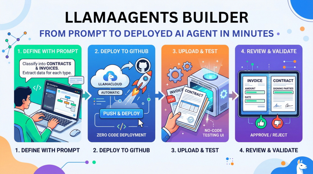
In this article, you will learn how to build, deploy, and test a no-code document-processing AI agent with LlamaAgents Builder in LlamaCloud. Topics we will cover include: How to create a document-classification agent using a natural language prompt. How to deploy the agent to a GitHub-backed application without writing code. How to test the deployed agent on invoices and contracts in the LlamaCloud interface. Let’s not waste any more time. LlamaAgents Builder: From Prompt to Deployed AI Agent in Minutes (click to enlarge)Image by Editor Introduction Creating an AI agent for tasks like analyzing and processing documents autonomously used to require hours of near-endless configuration, code orchestration, and deployment battles. Until now. This article unveils the process of building, deploying, and using an intelligent agent from scratch without writing a single line of code, using LlamaAgents Builder. Better still, we will host it as an app in a software repository that will be 100% owned by us. We will complete the whole process in a matter of minutes, so time is of the essence: let’s get started. Building with LlamaAgents Builder LlamaAgents Builder is one of the newest features in the LlamaCloud web platform, whose flagship product was originally introduced as LlamaParse. A slightly confusing mix of names, I know! For now, just keep in mind that we will access the agents builder through this link. The first thing you should see is a home menu like the one shown in the screenshot below. If this is not what you see, try clicking the “LlamaParse” icon in the top-left corner instead, and then you should see this — at least at the time of writing. LlamaParse home menu Notice that, in this example, we are working under a newly created free-plan account, which allows up to 10,000 pages of processing. See the “Agents” block on the bottom-right side? That is where LlamaAgents Builder lives. Even though it is in beta at the time of writing, we can already build useful agent-based workflows, as we will see. Once we click on it, a new screen will open with a chat interface similar to Gemini, ChatGPT, and others. You will get several suggested workflows for what you’d like your agent to do, but we will specify our own by typing the following prompt into the input box at the bottom. Just natural language, no code at all: Create an agent that classifies documents into “Contracts” and “Invoices”. For contracts, extract the signing parties; for invoices, the total amount and date. Specifying what the agent should do with a natural language prompt Simply send the prompt, and the magic will start. With a remarkable level of transparency in the reasoning process, you’ll see the steps completed and the progress made so far: AgentBuilder creating our agent workflow After a few minutes, the creation process will be complete. Not only can you see the full workflow diagram, which has gradually grown throughout the process, but you also receive a succinct and clear description of how to use your newly created agent. Simply amazing. Agent workflow built The next step is to deploy our agent so that it can be used. In the top-right corner, you may see a “Push & Deploy” button. This initiates the process of publishing your agent workflow’s software packages into a GitHub repository, so make sure you have a registered account on GitHub first. You can easily register with an existing Google or Microsoft account, for instance. Once you have the LlamaCloud platform connected to your GitHub account, it is extremely easy to push and deploy your agent: just give it a name, specify whether you want it in a private repository, and that’s it: Pushing and deploying agent workflow into GitHub The process will take a few minutes, and you will see a stream of command-line-like messages appearing on the fly. Once it is finalized and your agent status appears as “Running“, you will see a few final messages similar to this: [app] 10:01:08.583 info Application startup complete. (uvicorn.error) [app] 10:01:08.589 info Uvicorn running on http://0.0.0.0:8080 (Press CTRL+C to quit) (uvicorn.error) [app] 10:01:09.007 info HTTP Request: POST https://api.cloud.llamaindex.ai/api/v1/beta/agent-data/:search?project_id=<YOUR_PROJECT_ID_APPEARS_HERE> “HTTP/1.1 200 OK” (httpx) [app] 10:01:08.583 info Application startup complete. (uvicorn.error) [app] 10:01:08.589 info Uvicorn running on http://0.0.0.0:8080 (Press CTRL+C to quit) (uvicorn.error) [app] 10:01:09.007 info HTTP Request: POST https://api.cloud.llamaindex.ai/api/v1/beta/agent-data/:search?project_id=<YOUR_PROJECT_ID_APPEARS_HERE> “HTTP/1.1 200 OK” (httpx) The “Uvicorn” messages indicate that our agent has been deployed and is running as a microservice API within the LlamaCloud infrastructure. If you are familiar with FastAPI endpoints, you may want to try it programmatically through the API, but in this tutorial, we will keep things simpler (we promised zero coding, didn’t we?) and try everything ourselves in LlamaCloud’s own user interface. To do this, click the “Visit” button that appears at the top: Deployed agent up and running Now comes the most exciting part. You should have been taken to a playground page called “Review,” where you can try your agent out. Start by uploading a file, for example, a PDF document containing an invoice or a contract. If you don’t have one, just create a fictitious example document of your own using Microsoft Word, Google Docs, or a similar tool, such as this one: LlamaCloud Agent Testing UI: processing an invoice As soon as the document is loaded, the agent starts working on its own, and in a matter of seconds, it will classify your document and extract the required data fields, depending on the document type. You can see this result on the right-hand-side panel in the image above: the total amount and invoice date have been correctly extracted by the agent. How about uploading an example document containing a contract now? LlamaCloud Agent Testing UI: processing a contract As expected, the document is now classified as a contract, and on this occasion, the extracted information consists of the names of the signing parties. Well done! As you keep running examples, make sure you approve or reject them based on whether they have

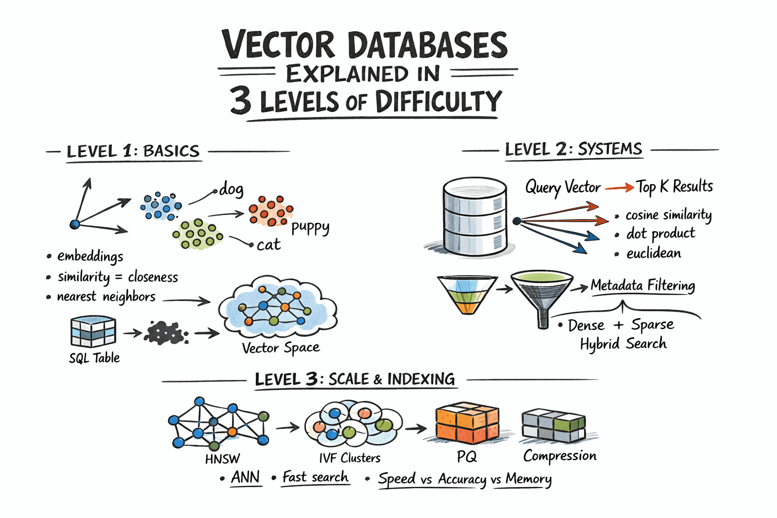
In this article, you will learn how vector databases work, from the basic idea of similarity search to the indexing strategies that make large-scale retrieval practical. Topics we will cover include: How embeddings turn unstructured data into vectors that can be searched by similarity. How vector databases support nearest neighbor search, metadata filtering, and hybrid retrieval. How indexing techniques such as HNSW, IVF, and PQ help vector search scale in production. Let’s not waste any more time. Vector Databases Explained in 3 Levels of DifficultyImage by Author Introduction Traditional databases answer a well-defined question: does the record matching these criteria exist? Vector databases answer a different one: which records are most similar to this? This shift matters because a huge class of modern data — documents, images, user behavior, audio — cannot be searched by exact match. So the right query is not “find this,” but “find what is close to this.” Embedding models make this possible by converting raw content into vectors, where geometric proximity corresponds to semantic similarity. The problem, however, is scale. Comparing a query vector against every stored vector means billions of floating-point operations at production data sizes, and that math makes real-time search impractical. Vector databases solve this with approximate nearest neighbor algorithms that skip the vast majority of candidates and still return results nearly identical to an exhaustive search, at a fraction of the cost. This article explains how that works at three levels: the core similarity problem and what vectors enable, how production systems store and query embeddings with filtering and hybrid search, and finally the indexing algorithms and architecture decisions that make it all work at scale. Level 1: Understanding the Similarity Problem Traditional databases store structured data — rows, columns, integers, strings — and retrieve it with exact lookups or range queries. SQL is fast and precise for this. But a lot of real-world data is not structured. Text documents, images, audio, and user behavior logs do not fit neatly into columns, and “exact match” is the wrong query for them. The solution is to represent this data as vectors: fixed-length arrays of floating-point numbers. An embedding model like OpenAI’s text-embedding-3-small, or a vision model for images, converts raw content into a vector that captures its semantic meaning. Similar content produces similar vectors. For example, the word “dog” and the word “puppy” end up geometrically close in vector space. A photo of a cat and a drawing of a cat also end up close. A vector database stores these embeddings and lets you search by similarity: “find me the 10 vectors closest to this query vector.” This is called nearest neighbor search. Level 2: Storing and Querying Vectors Embeddings Before a vector database can do anything, content needs to be converted into vectors. This is done by embedding models — neural networks that map input into a dense vector space, typically with 256 to 4096 dimensions depending on the model. The specific numbers in the vector do not have direct interpretations; what matters is the geometry: close vectors mean similar content. You call an embedding API or run a model yourself, get back an array of floats, and store that array alongside your document metadata. Distance Metrics Similarity is measured as geometric distance between vectors. Three metrics are common: Cosine similarity measures the angle between two vectors, ignoring magnitude. It is often used for text embeddings, where direction matters more than length. Euclidean distance measures straight-line distance in vector space. It is useful when magnitude carries meaning. Dot product is fast and works well when vectors are normalized. Many embedding models are trained to use it. The choice of metric should match how your embedding model was trained. Using the wrong metric degrades result quality. The Nearest Neighbor Problem Finding exact nearest neighbors is trivial in small datasets: compute the distance from the query to every vector, sort the results, and return the top K. This is called brute-force or flat search, and it is 100% accurate. It also scales linearly with dataset size. At 10 million vectors with 1536 dimensions each, a flat search is too slow for real-time queries. The solution is approximate nearest neighbor (ANN) algorithms. These trade a small amount of accuracy for large gains in speed. Production vector databases run ANN algorithms under the hood. The specific algorithms, their parameters, and their tradeoffs are what we will examine in the next level. Metadata Filtering Pure vector search returns the most semantically similar items globally. In practice, you usually want something closer to: “find the most similar documents that belong to this user and were created after this date.” That is hybrid retrieval: vector similarity combined with attribute filters. Implementations vary. Pre-filtering applies the attribute filter first, then runs ANN on the remaining subset. Post-filtering runs ANN first, then filters the results. Pre-filtering is more accurate but more expensive for selective queries. Most production databases use some variant of pre-filtering with smart indexing to keep it fast. Hybrid Search: Dense + Sparse Pure dense vector search can miss keyword-level precision. A query for “GPT-5 release date” might semantically drift toward general AI topics rather than the specific document containing the exact phrase. Hybrid search combines dense ANN with sparse retrieval (BM25 or TF-IDF) to get semantic understanding and keyword precision together. The standard approach is to run dense and sparse search in parallel, then combine scores using reciprocal rank fusion (RRF) — a rank-based merging algorithm that does not require score normalization. Most production systems now support hybrid search natively. Level 3: Indexing for Scale Approximate Nearest Neighbor Algorithms The three most important approximate nearest neighbor algorithms each occupy a different point on the tradeoff surface between speed, memory usage, and recall. Hierarchical navigable small world (HNSW) builds a multi-layer graph where each vector is a node, with edges connecting similar neighbors. Higher layers are sparse and enable fast long-range traversal; lower layers are denser for precise local search. At query time, the algorithm hops through

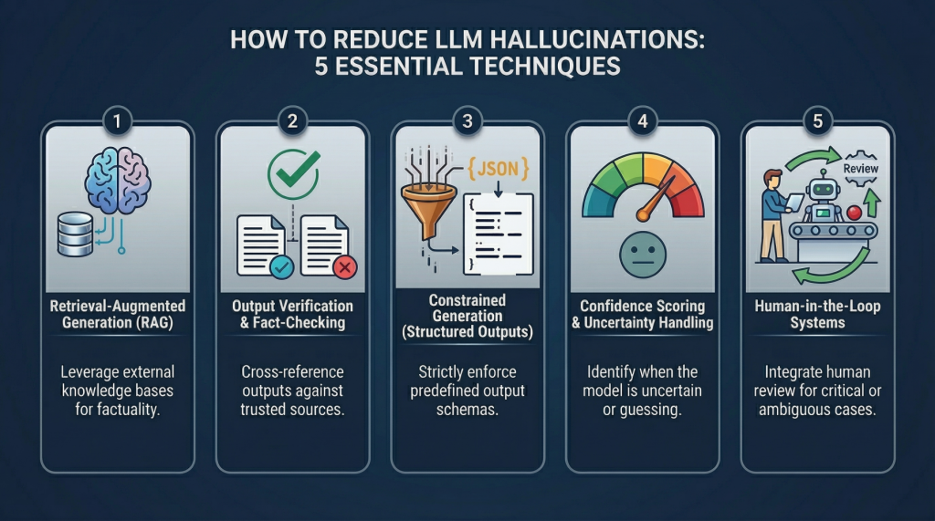
5 Practical Techniques to Detect and Mitigate LLM Hallucinations Beyond Prompt Engineering – MachineLearningMastery.com 5 Practical Techniques to Detect and Mitigate LLM Hallucinations Beyond Prompt Engineering – MachineLearningMastery.com

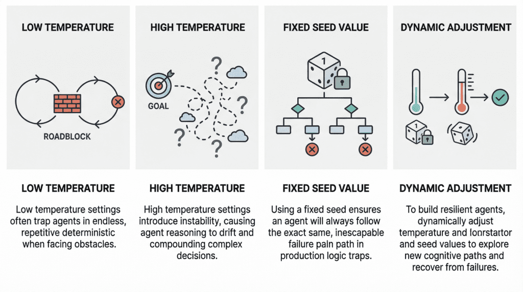
In this article, you will learn how temperature and seed values influence failure modes in agentic loops, and how to tune them for greater resilience. Topics we will cover include: How low and high temperature settings can produce distinct failure patterns in agentic loops. Why fixed seed values can undermine robustness in production environments. How to use temperature and seed adjustments to build more resilient and cost-effective agent workflows. Let’s not waste any more time. Why Agents Fail: The Role of Seed Values and Temperature in Agentic LoopsImage by Editor Introduction In the modern AI landscape, an agent loop is a cyclic, repeatable, and continuous process whereby an entity called an AI agent — with a certain degree of autonomy — works toward a goal. In practice, agent loops now wrap a large language model (LLM) inside them so that, instead of reacting only to single-user prompt interactions, they implement a variation of the Observe-Reason-Act cycle defined for classic software agents decades ago. Agents are, of course, not infallible, and they may sometimes fail, in some cases due to poor prompting or a lack of access to the external tools they need to reach a goal. However, two invisible steering mechanisms can also influence failure: temperature and seed value. This article analyzes both from the perspective of failure in agent loops. Let’s take a closer look at how these settings may relate to failure in agentic loops through a gentle discussion backed by recent research and production diagnoses. Temperature: “Reasoning Drift” Vs. “Deterministic Loop” Temperature is an inherent parameter of LLMs, and it controls randomness in their internal behavior when selecting the words, or tokens, that make up the model’s response. The higher its value (closer to 1, assuming a range between 0 and 1), the less deterministic and more unpredictable the model’s outputs become, and vice versa. In agentic loops, because LLMs sit at the core, understanding temperature is crucial to understanding unique, well-documented failure modes that may arise, particularly when the temperature is extremely low or high. A low-temperature (near 0) agent often yields the so-called deterministic loop failure. In other words, the agent’s behavior becomes too rigid. Suppose the agent comes across a “roadblock” on its path, such as a third-party API consistently returning an error. With a low temperature and exceedingly deterministic behavior, it lacks the kind of cognitive randomness or exploration needed to pivot. Recent studies have scientifically analyzed this phenomenon. The practical consequences typically observed range from agents finalizing missions prematurely to failing to coordinate when their initial plans encounter friction, thus ending up in loops of the same attempts over and over without any progress. At the opposite end of the spectrum, we have high-temperature (0.8 or above) agentic loops. As with standalone LLMs, high temperature introduces a much broader range of possibilities when sampling each element of the response. In a multi-step loop, however, this highly probabilistic behavior may compound in a dangerous way, turning into a trait known as reasoning drift. In essence, this behavior boils down to instability in decision-making. Introducing high-temperature randomness into complex agent workflows may cause agent-based models to lose their way — that is, lose their original selection criteria for making decisions. This may include symptoms such as hallucinations (fabricated reasoning chains) or even forgetting the user’s initial goal. Seed Value: Reproducibility Seed values are the mechanisms that initialize the pseudo-random generator used to build the model’s outputs. Put more simply, the seed value is like the starting position of a die that is rolled to kickstart the model’s word-selection mechanism governing response generation. Regarding this setting, the main problem that usually causes failure in agent loops is using a fixed seed in production. A fixed seed is reasonable in a testing environment, for example, for the sake of reproducibility in tests and experiments, but allowing it to make its way into production introduces a significant vulnerability. An agent may inadvertently enter a logic trap when it operates with a fixed seed. In such a situation, the system may automatically trigger a recovery attempt, but even then, the fixed seed is almost synonymous with guaranteeing that the agent will take the same reasoning path doomed to failure over and over again. In practical terms, imagine an agent tasked with debugging a failed deployment by inspecting logs, proposing a fix, and then retrying the operation. If the loop runs with a fixed seed, the stochastic choices made by the model during each reasoning step may remain effectively “locked” into the same pattern every time recovery is triggered. As a result, the agent may keep selecting the same flawed interpretation of the logs, calling the same tool in the same order, or generating the same ineffective fix despite repeated retries. What looks like persistence at the system level is, in reality, repetition at the cognitive level. This is why resilient agent architectures often treat the seed as a controllable recovery lever: when the system detects that the agent is stuck, changing the seed can help force exploration of a different reasoning trajectory, increasing the chances of escaping a local failure mode rather than reproducing it indefinitely. A summary of the role of seed values and temperature in agentic loopsImage by Editor Best Practices For Resilient And Cost-Effective Loops Having learned about the impact that temperature and seed value may have in agent loops, one might wonder how to make these loops more resilient to failure by carefully setting these two parameters. Basically, breaking out of failure in agentic loops often entails changing the seed value or temperature as part of retry efforts to seek a different cognitive path. Resilient agents usually implement approaches that dynamically adjust these parameters in edge cases, for instance by temporarily raising the temperature or randomizing the seed if an analysis of the agent’s state suggests it is stuck. The bad news is that this can become very expensive to test when commercial APIs are used, which is why open-weight models, local models,