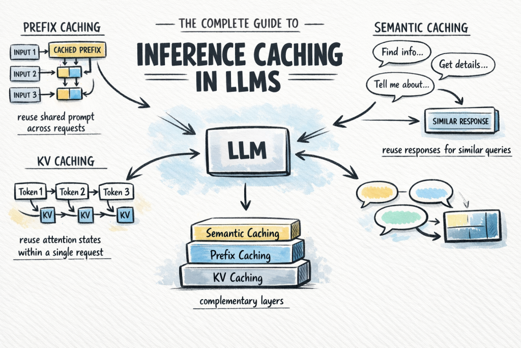
In this article, you will learn how inference caching works in large language models and how to use it to reduce cost and latency in production systems. Topics we will cover include: The fundamentals of inference caching and why it matters The three main caching types: KV caching, prefix caching, and semantic caching How to choose and combine caching strategies in real-world applications The Complete Guide to Inference Caching in LLMsImage by Author Introduction Calling a large language model API at scale is expensive and slow. A significant share of that cost comes from repeated computation: the same system prompt processed from scratch on every request, and the same common queries answered as if the model has never seen them before. Inference caching addresses this by storing the results of expensive LLM computations and reusing them when an equivalent request arrives. Depending on which caching layer you apply, you can skip redundant attention computation mid-request, avoid reprocessing shared prompt prefixes across requests, or serve common queries from a lookup without invoking the model at all. In production systems, this can significantly reduce token spend with almost no change to application logic. This article covers: What inference caching is and why it matters The three main caching types: key-value (KV), prefix, and semantic caching How semantic caching extends coverage beyond exact prefix matches Each section builds toward a practical decision framework for choosing the right caching strategy for your application. What Is Inference Caching? When you send a prompt to a large language model, the model performs a substantial amount of computation to process the input and generate each output token. That computation takes time and costs money. Inference caching is the practice of storing the results of that computation — at various levels of granularity — and reusing them when a similar or identical request arrives. There are three distinct types to understand, each operating at a different layer of the stack: KV caching: Caches the internal attention states — key-value pairs — computed during a single inference request, so the model does not recompute them at every decode step. This happens automatically inside the model and is always on. Prefix caching: Extends KV caching across multiple requests. When different requests share the same leading tokens, such as a system prompt, a reference document, or few-shot examples, the KV states for that shared prefix are stored and reused across all of them. You may also see this called prompt caching or context caching. Semantic caching: A higher-level, application-side cache that stores complete LLM input/output pairs and retrieves them based on semantic similarity. Unlike prefix caching, which operates on attention states mid-computation, semantic caching short-circuits the model call entirely when a sufficiently similar query has been seen before. These are not interchangeable alternatives. They are complementary layers. KV caching is always running. Prefix caching is the highest-leverage optimization you can add to most production applications. Semantic caching is a further enhancement when query volume and similarity are high enough to justify it. Understanding How KV Caching Works KV caching is the foundation that everything else builds on. To understand it, you need a brief look at how transformer attention works during inference. The Attention Mechanism and Its Cost Modern LLMs use the transformer architecture with self-attention. For every token in the input, the model computes three vectors: Q (Query) — What is this token looking for? K (Key) — What does this token offer to other tokens? V (Value) — What information does this token carry? Attention scores are computed by comparing each token’s query against the keys of all previous tokens, then using those scores to weight the values. This allows the model to understand context across the full sequence. LLMs generate output autoregressively — one token at a time. Without caching, generating token N would require recomputing K and V for all N-1 previous tokens from scratch. For long sequences, this cost compounds with every decode step. How KV Caching Fixes This During a forward pass, once the model computes the K and V vectors for a token, those values are saved in GPU memory. For each subsequent decode step, the model looks up the stored K and V pairs for the existing tokens rather than recomputing them. Only the newly generated token requires fresh computation. Here is a simple example: Without KV caching (generating token 100): Recompute K, V for tokens 1–99 → then compute token 100 With KV caching (generating token 100): Load stored K, V for tokens 1–99 → compute token 100 only Without KV caching (generating token 100): Recompute K, V for tokens 1–99 → then compute token 100   With KV caching (generating token 100): Load stored K, V for tokens 1–99 → compute token 100 only This is KV caching in its original sense: an optimization within a single request. It is automatic and universal; every LLM inference framework enables it by default. You do not need to configure it. However, understanding it is essential for understanding prefix caching, which extends this mechanism across requests. For a more thorough explanation, see KV Caching in LLMs: A Guide for Developers. Using Prefix Caching to Reuse KV States Across Requests Prefix caching — also called prompt caching or context caching depending on the provider — takes the KV caching concept one step further. Instead of caching attention states only within a single request, it caches them across multiple requests — specifically for any shared prefix those requests have in common. The Core Idea Consider a typical production LLM application. You have a long system prompt — instructions, a reference document, and few-shot examples — that is identical across every request. Only the user’s message at the end changes. Without prefix caching, the model recomputes the KV states for that entire system prompt on every call. With prefix caching, it computes them once, stores them, and every subsequent request that shares that prefix skips directly to processing the user’s message. The Hard Requirement: Exact

In this article, you will learn how to use Python decorators to improve the reliability, observability, and efficiency of machine learning systems in production. Topics we will cover include: Implementing retry logic with exponential backoff for unstable external dependencies. Validating inputs and enforcing schemas before model inference. Optimizing performance with caching, memory guards, and monitoring decorators. Python Decorators for Production ML EngineeringImage by Editor Introduction You’ve probably written a decorator or two in your Python career. Maybe a simple @timer to benchmark a function, or a @login_required borrowed from Flask. But decorators become a completely different animal once you’re running machine learning models in production. Suddenly, you’re dealing with flaky API calls, memory leaks from massive tensors, input data that drifts without warning, and functions that need to fail gracefully at 3 AM when nobody’s watching. The five decorators in this article aren’t textbook examples. They’re patterns that solve real, recurring headaches in production machine learning systems, and they will change how you think about writing resilient inference code. 1. Automatic Retry with Exponential Backoff Production machine learning pipelines constantly interact with external services. You might be calling a model endpoint, pulling embeddings from a vector database, or fetching features from a remote store. These calls fail. Networks hiccup, services throttle requests, and cold starts introduce latency spikes. Wrapping every call in try/except blocks with retry logic quickly turns your codebase into a mess. Fortunately, @retry solves this elegantly. You define the decorator to accept parameters such as max_retries, backoff_factor, and a tuple of retriable exceptions. Inside, the wrapper function catches those specific exceptions, waits using exponential backoff (multiplying the delay after each attempt), and re-raises the exception if all retries are exhausted. The advantage here is that your core function remains clean. It simply performs the call. The resilience logic is centralized, and you can tune retry behavior per function through decorator arguments. For model-serving endpoints that occasionally experience timeouts, this single decorator can mean the difference between noisy alerts and seamless recovery. 2. Input Validation and Schema Enforcement Data quality issues are a silent failure mode in machine learning systems. Models are trained on features with specific distributions, types, and ranges. In production, upstream changes can introduce null values, incorrect data types, or unexpected shapes. By the time you detect the issue, your system may have been serving poor predictions for hours. A @validate_input decorator intercepts function arguments before they reach your model logic. You can design it to check whether a NumPy array matches an expected shape, whether required dictionary keys are present, or whether values fall within acceptable ranges. When validation fails, the decorator raises a descriptive error or returns a safe default response instead of allowing corrupted data to propagate downstream. This pattern pairs well with Pydantic if you want more sophisticated validation. However, even a lightweight implementation that checks array shapes and data types before inference will prevent many common production issues. It is a proactive defense rather than reactive debugging. 3. Result Caching with TTL If you are serving predictions in real time, you will encounter repeated inputs. For example, the same user may hit a recommendation endpoint multiple times in a session, or a batch job may reprocess overlapping feature sets. Running inference repeatedly wastes compute resources and adds unnecessary latency. A @cache_result decorator with a time-to-live (TTL) parameter stores function outputs keyed by their inputs. Internally, you maintain a dictionary mapping hashed arguments to tuples of (result, timestamp). Before executing the function, the wrapper checks whether a valid cached result exists. If the entry is still within the TTL window, it returns the cached value. Otherwise, it executes the function and updates the cache. The TTL component makes this approach production-ready. Predictions can become stale, especially when underlying features change. You want caching, but with an expiration policy that reflects how quickly your data evolves. In many real-time scenarios, even a short TTL of 30 seconds can significantly reduce redundant computation. 4. Memory-Aware Execution Large models consume significant memory. When running multiple models or processing large batches, it is easy to exceed available RAM and crash your service. These failures are often intermittent, depending on workload variability and garbage collection timing. A @memory_guard decorator checks available system memory before executing a function. Using psutil, it reads current memory usage and compares it against a configurable threshold (for example, 85% utilization). If memory is constrained, the decorator can trigger garbage collection with gc.collect(), log a warning, delay execution, or raise a custom exception that an orchestration layer can handle gracefully. This is especially useful in containerized environments, where memory limits are strict. Platforms such as Kubernetes will terminate your service if it exceeds its memory allocation. A memory guard gives your application an opportunity to degrade gracefully or recover before reaching that point. 5. Execution Logging and Monitoring Observability in machine learning systems extends beyond HTTP status codes. You need visibility into inference latency, anomalous inputs, shifting prediction distributions, and performance bottlenecks. While ad hoc logging works initially, it becomes inconsistent and difficult to maintain as systems grow. A @monitor decorator wraps functions with structured logging that captures execution time, input summaries, output characteristics, and exception details automatically. It can integrate with logging frameworks, Prometheus metrics, or observability platforms such as Datadog. The decorator timestamps execution start and end, logs exceptions before re-raising them, and optionally pushes metrics to a monitoring backend. The real value emerges when this decorator is applied consistently across the inference pipeline. You gain a unified, searchable record of predictions, execution times, and failures. When issues arise, engineers have actionable context instead of limited diagnostic information. Final Thoughts These five decorators share a common philosophy: keep core machine learning logic clean while pushing operational concerns to the edges. Decorators provide a natural separation that improves readability, testability, and maintainability. Start with the decorator that addresses your most immediate challenge. For many teams, that is retry logic or monitoring. Once you experience the clarity this pattern brings, it

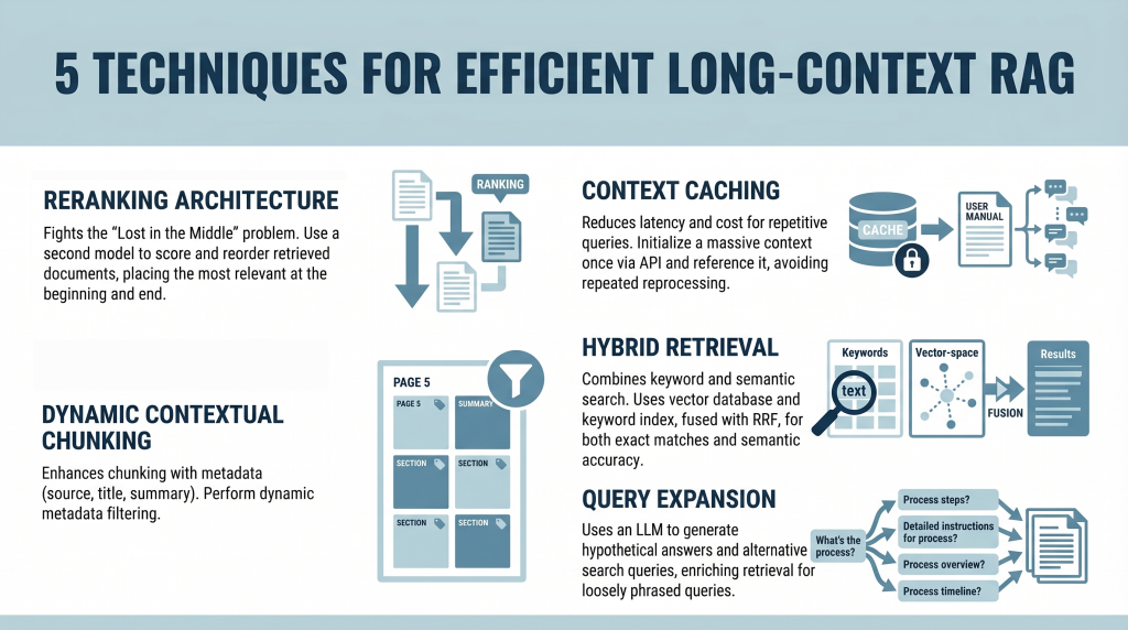
In this article, you will learn how to build efficient long-context retrieval-augmented generation (RAG) systems using modern techniques that address attention limitations and cost challenges. Topics we will cover include: How reranking mitigates the “Lost in the Middle” problem. How context caching reduces latency and computational cost. How hybrid retrieval, metadata filtering, and query expansion improve relevance. Introduction Retrieval-augmented generation (RAG) is undergoing a major shift. For years, the RAG mantra was simple: “Break your documents into smaller pieces, embed them, and retrieve the most relevant pieces.” This was necessary because large language models (LLMs) had context windows that were expensive and limited, typically ranging from 4,000 to 32,000 tokens. Now, models like Gemini Pro and Claude Opus have broken these limits, offering context windows of 1 million tokens or more. In theory, you could now paste an entire collection of novels into a prompt. In practice, however, this capability introduces two major challenges: The “Lost in the Middle” Problem: Research has shown that models often ignore information placed in the middle of a massive prompt, favoring the beginning and the end. The Cost Problem: Processing a million tokens for every query is computationally expensive and slow. It’s like rereading an entire encyclopedia every time someone asks a simple question. This tutorial explores five practical techniques for building efficient long-context RAG systems. We move beyond simple partitioning and examine strategies for mitigating attention loss and enabling context reuse from a developer’s perspective. 1. Implementing a Reranking Architecture to Fight “Lost in the Middle” The “Lost in the Middle” problem, identified in a 2023 study by Stanford and UC Berkeley, reveals a critical limitation in LLM attention mechanisms. When presented with long context, model performance peaks when relevant information appears at the beginning or end. Information buried in the middle is significantly more likely to be ignored or misinterpreted. Instead of inserting retrieved documents directly into the prompt in their original order, introduce a reranking step. Here is the developer workflow: Retrieval: Use a standard vector database (such as Pinecone or Weaviate) to retrieve a larger candidate set (e.g. top 20 instead of top 5) Reranking: Pass these candidates through a specialized cross-encoder reranker (such as the Cohere Rerank API or a Sentence-Transformers cross-encoder model) that scores each document against the query Reordering: Select the top 5 most relevant documents Context Placement: Place the most relevant document at the beginning and the second-most relevant at the end of the prompt. Position the remaining three in the middle This strategic placement ensures that the most important information receives maximum attention. 2. Leveraging Context Caching for Repetitive Queries Long contexts introduce latency and cost overhead. Processing hundreds of thousands of tokens repeatedly is inefficient. Context caching addresses this issue. Think of this as initializing a persistent context for your model. Create the Cache: Upload a large document (e.g. a 500,000-token manual) once via an API and define a time-to-live (TTL) Reference the Cache: For subsequent queries, send only the user’s question along with a reference ID to the cached context Cost Savings: You reduce input token costs and latency, since the document does not need to be reprocessed each time This approach is especially useful for chatbots built on static knowledge bases. 3. Using Dynamic Contextual Chunking with Metadata Filters Even with large context windows, relevance remains critical. Simply increasing context size does not eliminate noise. This approach enhances traditional chunking with structured metadata. Intelligent Chunking: Split documents into segments (e.g. 500–1000 tokens) and attach metadata such as source, section title, page number, and summaries Hybrid Filtering: Use a two-step retrieval process: Metadata Filtering: Narrow the search space based on structured attributes (e.g. date ranges or document sections) Semantic Search: Perform similarity search only on filtered candidates This reduces irrelevant context and improves precision. 4. Combining Keyword and Semantic Search with Hybrid Retrieval Vector search captures meaning but can miss exact keyword matches, which are essential for technical queries. Hybrid search combines semantic and keyword-based retrieval. Dual Retrieval: Vector database for semantic similarity Keyword index (e.g. Elasticsearch) for exact matches Fusion: Use Reciprocal Rank Fusion (RRF) to combine rankings, prioritizing results that score highly in both systems Context Population: Insert the fused results into the prompt using reranking principles This ensures both semantic relevance and lexical accuracy. 5. Applying Query Expansion with Summarize-Then-Retrieve User queries often differ from how information is expressed in documents. Query expansion helps bridge this gap. Use a lightweight LLM to generate alternative search queries. This improves performance on inferential and loosely phrased queries. Conclusion The emergence of million-token context windows does not eliminate the need for retrieval-augmented generation—it reshapes it. While long contexts reduce the need for aggressive chunking, they introduce challenges related to attention distribution and cost. By applying reranking, context caching, metadata filtering, hybrid retrieval, and query expansion, you can build systems that are both scalable and precise. The goal is not simply to provide more context, but to ensure the model consistently focuses on the most relevant information. References How Language Models Use Long Contexts Gemini API: Context Caching Rerank – The Power of Semantic Search (Cohere) The Probabilistic Relevance Framework About Shittu Olumide Shittu Olumide is a software engineer and technical writer passionate about leveraging cutting-edge technologies to craft compelling narratives, with a keen eye for detail and a knack for simplifying complex concepts. You can also find Shittu on Twitter.

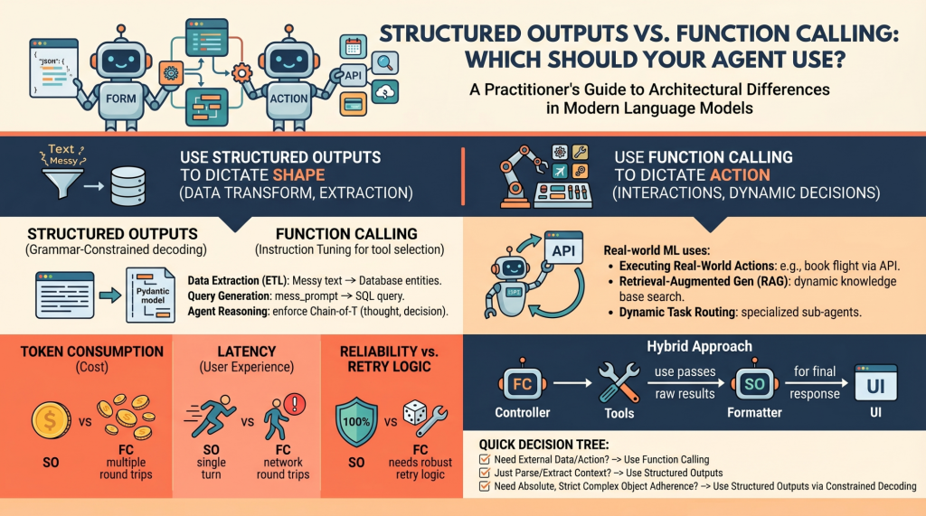
In this article, you will learn the architectural differences between structured outputs and function calling in modern language model systems. Topics we will cover include: How structured outputs and function calling work under the hood. When to use each approach in real-world machine learning systems. The performance, cost, and reliability trade-offs between the two. Structured Outputs vs. Function Calling: Which Should Your Agent Use?Image by Editor Introduction Language models (LMs), at their core, are text-in and text-out systems. For a human conversing with one via a chat interface, this is perfectly fine. But for machine learning practitioners building autonomous agents and reliable software pipelines, raw unstructured text is a nightmare to parse, route, and integrate into deterministic systems. To build reliable agents, we need predictable, machine-readable outputs and the ability to interact seamlessly with external environments. In order to bridge this gap, modern LM API providers (like OpenAI, Anthropic, and Google Gemini) have introduced two primary mechanisms: Structured Outputs: Forcing the model to reply by adhering exactly to a predefined schema (most commonly a JSON schema or a Python Pydantic model) Function Calling (Tool Use): Equipping the model with a library of functional definitions that it can choose to invoke dynamically based on the context of the prompt At first glance, these two capabilities look very similar. Both typically rely on passing JSON schemas to the API under the hood, and both result in the model outputting structured key-value pairs instead of conversational prose. However, they serve fundamentally different architectural purposes in agent design. Conflating the two is a common pitfall. Choosing the wrong mechanism for a feature can lead to brittle architectures, excessive latency, and unnecessarily inflated API costs. Let’s unpack the architectural distinctions between these methods and provide a decision-making framework for when to use each. Unpacking the Mechanics: How They Work Under the Hood To understand when to use these features, it is necessary to understand how they differ at the mechanical and API levels. Structured Outputs Mechanics Historically, getting a model to output raw JSON relied on prompt engineering (“You are a helpful assistant that *only* speaks in JSON…”). This was error-prone, requiring extensive retry logic and validation. Modern “structured outputs” fundamentally change this through grammar-constrained decoding. Libraries like Outlines, or native features like OpenAI’s Structured Outputs, mathematically restrict the token probabilities at generation time. If the chosen schema dictates that the next token must be a quotation mark or a specific boolean value, the probabilities of all non-compliant tokens are masked out (set to zero). This is a single-turn generation strictly focused on form. The model is answering the prompt directly, but its vocabulary is confined to the exact structure you defined, with the aim of ensuring near 100% schema compliance. Function Calling Mechanics Function calling, on the other hand, relies heavily on instruction tuning. During training, the model is fine-tuned to recognize situations where it lacks the necessary information to complete a prompt, or when the prompt explicitly asks it to take an action. When you provide a model with a list of tools, you are telling it, “If you need to, you can pause your text generation, select a tool from this list, and generate the necessary arguments to run it.” This is an inherently multi-turn, interactive flow: The model decides to call a tool and outputs the tool name and arguments. The model pauses. It cannot execute the code itself. Your application code executes the selected function locally using the generated arguments. Your application returns the result of the function back to the model. The model synthesizes this new information and continues generating its final response. When to Choose Structured Outputs Structured outputs should be your default approach whenever the goal is pure data transformation, extraction, or standardization. Primary Use Case: The model has all the necessary information within the prompt and context window; it just needs to reshape it. Examples for Practitioners: Data Extraction (ETL): Processing raw, unstructured text like a customer support transcript and extracting entities &emdash; names, dates, complaint types, and sentiment scores &emdash; into a strict database schema. Query Generation: Converting a messy natural language user prompt into a strict, validated SQL query or a GraphQL payload. If the schema is broken, the query fails, making 100% adherence critical. Internal Agent Reasoning: Structuring an agent’s “thoughts” before it acts. You can enforce a Pydantic model that requires a thought_process field, an assumptions field, and finally a decision field. This forces a Chain-of-Thought process that is easily parsed by your backend logging systems. The Verdict: Use structured outputs when the “action” is simply formatting. Because there is no mid-generation interaction with external systems, this approach ensures high reliability, lower latency, and zero schema-parsing errors. When to Choose Function Calling Function calling is the engine of agentic autonomy. If structured outputs dictate the shape of the data, function calling dictates the control flow of the application. Primary Use Case: External interactions, dynamic decision-making, and cases where the model needs to fetch information it doesn’t currently possess. Examples for Practitioners: Executing Real-World Actions: Triggering external APIs based on conversational intent. If a user says, “Book my usual flight to New York,” the model uses function calling to trigger the book_flight(destination=”JFK”) tool. Retrieval-Augmented Generation (RAG): Instead of a naive RAG pipeline that always searches a vector database, an agent can use a search_knowledge_base tool. The model dynamically decides what search terms to use based on the context, or decides not to search at all if it already knows the answer. Dynamic Task Routing: For complex systems, a router model might use function calling to select the best specialized sub-agent (e.g., calling delegate_to_billing_agent versus delegate_to_tech_support) to handle a specific query. The Verdict: Choose function calling when the model must interact with the outside world, fetch hidden data, or conditionally execute software logic mid-thought. Performance, Latency, and Cost Implications When deploying agents to production, the architectural choice between these two methods directly impacts your unit economics and user experience. Token Consumption: Function calling

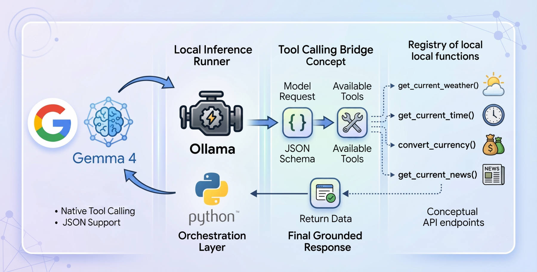
In this article, you will learn how to build a local, privacy-first tool-calling agent using the Gemma 4 model family and Ollama. Topics we will cover include: An overview of the Gemma 4 model family and its capabilities. How tool calling enables language models to interact with external functions. How to implement a local tool calling system using Python and Ollama. How to Implement Tool Calling with Gemma 4 and PythonImage by Editor Introducing the Gemma 4 Family The open-weights model ecosystem shifted recently with the release of the Gemma 4 model family. Built by Google, the Gemma 4 variants were created with the intention of providing frontier-level capabilities under a permissive Apache 2.0 license, enabling machine learning practitioners complete control over their infrastructure and data privacy. The Gemma 4 release features models ranging from the parameter-dense 31B and structurally complex 26B Mixture of Experts (MoE) to lightweight, edge-focused variants. More importantly for AI engineers, the model family features native support for agentic workflows. They have been fine-tuned to reliably generate structured JSON outputs and natively invoke function calls based on system instructions. This transforms them from “fingers crossed” reasoning engines into practical systems capable of executing workflows and conversing with external APIs locally. Tool Calling in Language Models Language models began life as closed-loop conversationalists. If you asked a language model for real-world sensor reading or live market rates, it could at best apologize, and at worst, hallucinate an answer. Tool calling, aka function calling, is the foundational architecture shift required to fix this gap. Tool calling serves as the bridge that can help transform static models into dynamic autonomous agents. When tool calling is enabled, the model evaluates a user prompt against a provided registry of available programmatic tools (supplied via JSON schema). Rather than attempting to guess the answer using only internal weights, the model pauses inference, formats a structured request specifically designed to trigger an external function, and awaits the result. Once the result is processed by the host application and handed back to the model, the model synthesizes the injected live context to formulate a grounded final response. The Setup: Ollama and Gemma 4:E2B To build a genuinely local, private-first tool calling system, we will use Ollama as our local inference runner, paired with the gemma4:e2b (Edge 2 billion parameter) model. The gemma4:e2b model is built specifically for mobile devices and IoT applications. It represents a paradigm shift in what is possible on consumer hardware, activating an effective 2 billion parameter footprint during inference. This optimization preserves system memory while achieving near-zero latency execution. By executing entirely offline, it removes rate limits and API costs while preserving strict data privacy. Despite this incredibly small size, Google has engineered gemma4:e2b to inherit the multimodal properties and native function-calling capabilities of the larger 31B model, making it an ideal foundation for a fast, responsive desktop agent. It also allows us to test for the capabilities of the new model family without requiring a GPU. The Code: Setting Up the Agent To orchestrate the language model and the tool interfaces, we will rely on a zero-dependency philosophy for our implementation, leveraging only standard Python libraries like urllib and json, ensuring maximum portability and transparency while also avoiding bloat. The complete code for this tutorial can be found at this GitHub repository. The architectural flow of our application operates in the following way: Define local Python functions that act as our tools Define a strict JSON schema that explains to the language model exactly what these tools do and what parameters they expect Pass the user’s query and the tool registry to the local Ollama API Catch the model’s response, identify if it requested a tool call, execute the corresponding local code, and feed the answer back Building the Tools: get_current_weather Let’s dive into the code, keeping in mind that our agent’s capability rests on the quality of its underlying functions. Our first function is get_current_weather, which reaches out to the open-source Open-Meteo API to resolve real-time weather data for a specific location. def get_current_weather(city: str, unit: str = “celsius”) -> str: “””Gets the current temperature for a given city using open-meteo API.””” try: # Geocode the city to get latitude and longitude geo_url = f”https://geocoding-api.open-meteo.com/v1/search?name={urllib.parse.quote(city)}&count=1″ geo_req = urllib.request.Request(geo_url, headers={‘User-Agent’: ‘Gemma4ToolCalling/1.0’}) with urllib.request.urlopen(geo_req) as response: geo_data = json.loads(response.read().decode(‘utf-8’)) if “results” not in geo_data or not geo_data[“results”]: return f”Could not find coordinates for city: {city}.” location = geo_data[“results”][0] lat = location[“latitude”] lon = location[“longitude”] country = location.get(“country”, “”) # Fetch the weather temp_unit = “fahrenheit” if unit.lower() == “fahrenheit” else “celsius” weather_url = f”https://api.open-meteo.com/v1/forecast?latitude={lat}&longitude={lon}&current=temperature_2m,wind_speed_10m&temperature_unit={temp_unit}” weather_req = urllib.request.Request(weather_url, headers={‘User-Agent’: ‘Gemma4ToolCalling/1.0’}) with urllib.request.urlopen(weather_req) as response: weather_data = json.loads(response.read().decode(‘utf-8’)) if “current” in weather_data: current = weather_data[“current”] temp = current[“temperature_2m”] wind = current[“wind_speed_10m”] temp_unit_str = weather_data[“current_units”][“temperature_2m”] wind_unit_str = weather_data[“current_units”][“wind_speed_10m”] return f”The current weather in {city.title()} ({country}) is {temp}{temp_unit_str} with wind speeds of {wind}{wind_unit_str}.” else: return f”Weather data for {city} is unavailable from the API.” except Exception as e: return f”Error fetching weather for {city}: {e}” 1 2 3 4 5 6 7 8 9 10 11 12 13 14 15 16 17 18 19 20 21 22 23 24 25 26 27 28 29 30 31 32 33 34 35 36 37 def get_current_weather(city: str, unit: str = “celsius”) -> str:     “”“Gets the current temperature for a given city using open-meteo API.”“”     try:         # Geocode the city to get latitude and longitude         geo_url = f“https://geocoding-api.open-meteo.com/v1/search?name={urllib.parse.quote(city)}&count=1”         geo_req = urllib.request.Request(geo_url, headers={‘User-Agent’: ‘Gemma4ToolCalling/1.0’})         with urllib.request.urlopen(geo_req) as response:             geo_data = json.loads(response.read().decode(‘utf-8’))           if “results” not in geo_data or not geo_data[“results”]:             return f“Could not find coordinates for city: {city}.”           location = geo_data[“results”][0]         lat = location[“latitude”]         lon = location[“longitude”]         country = location.get(“country”, “”)           # Fetch the weather         temp_unit = “fahrenheit” if unit.lower() == “fahrenheit” else “celsius”         weather_url = f“https://api.open-meteo.com/v1/forecast?latitude={lat}&longitude={lon}&current=temperature_2m,wind_speed_10m&temperature_unit={temp_unit}”         weather_req = urllib.request.Request(weather_url, headers={‘User-Agent’: ‘Gemma4ToolCalling/1.0’})         with urllib.request.urlopen(weather_req) as response:             weather_data = json.loads(response.read().decode(‘utf-8’))           if “current” in weather_data:             current = weather_data[“current”]             temp = current[“temperature_2m”]             wind = current[“wind_speed_10m”]             temp_unit_str = weather_data[“current_units”][“temperature_2m”]             wind_unit_str = weather_data[“current_units”][“wind_speed_10m”]

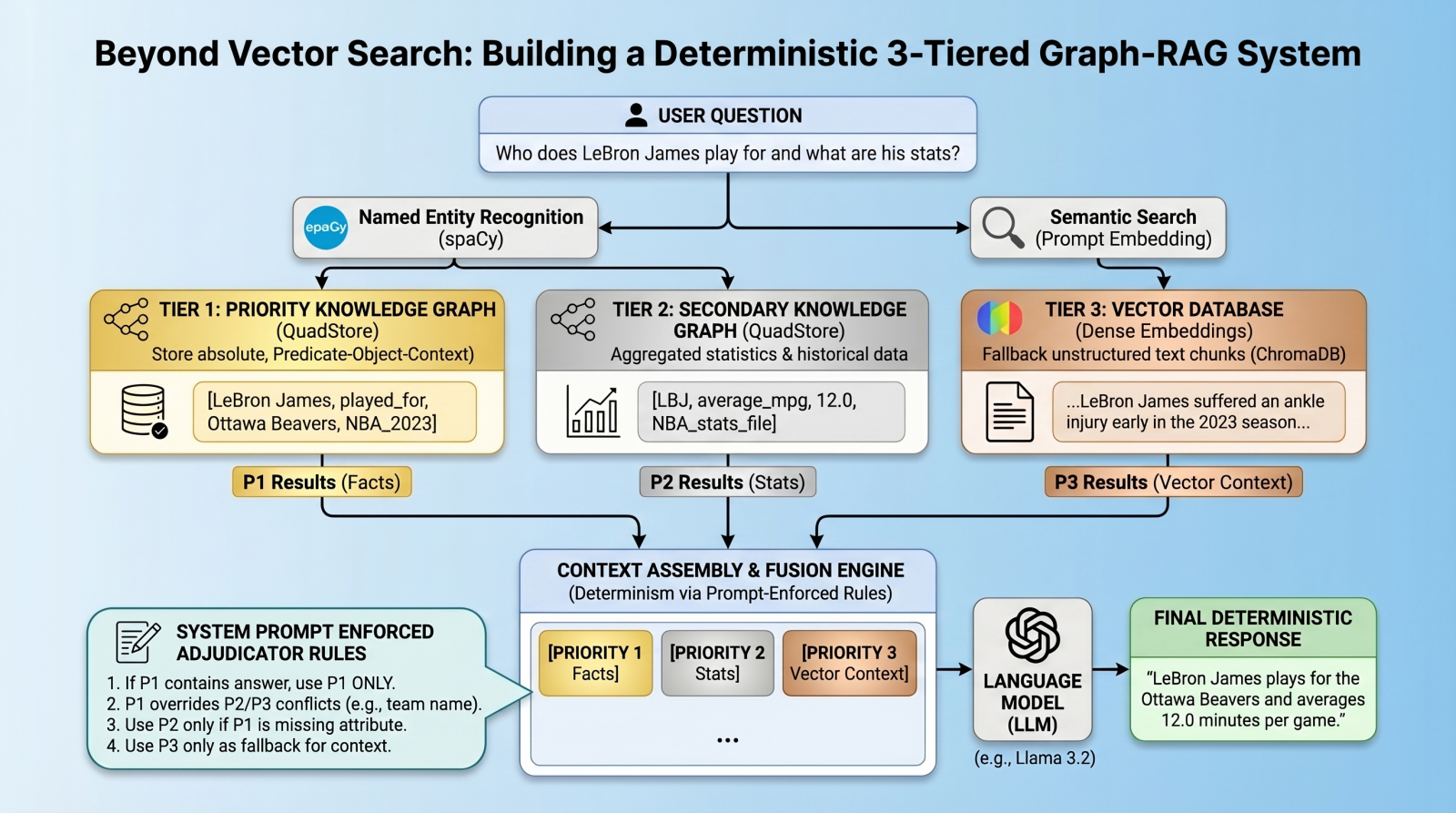
In this article, you will learn how to build a deterministic, multi-tier retrieval-augmented generation system using knowledge graphs and vector databases. Topics we will cover include: Designing a three-tier retrieval hierarchy for factual accuracy. Implementing a lightweight knowledge graph. Using prompt-enforced rules to resolve retrieval conflicts deterministically. Beyond Vector Search: Building a Deterministic 3-Tiered Graph-RAG SystemImage by Editor Introduction: The Limits of Vector RAG Vector databases have long since become the cornerstone of modern retrieval augmented generation (RAG) pipelines, excelling at retrieving long-form text based on semantic similarity. However, vector databases are notoriously “lossy” when it comes to atomic facts, numbers, and strict entity relationships. A standard vector RAG system might easily confuse which team a basketball player currently plays for, for example, simply because multiple teams appear near the player’s name in latent space. To solve this, we need a multi-index, federated architecture. In this tutorial, we will introduce such an architecture, using a quad store backend to implement a knowledge graph for atomic facts, backed by a vector database for long-tail, fuzzy context. But here is the twist: instead of relying on complex algorithmic routing to pick the right database, we will query all databases, dump the results into the context window, and use prompt-enforced fusion rules to force the language model (LM) to deterministically resolve conflicts. The goal is to attempt to eliminate relationship hallucinations and build absolute deterministic predictability where it matters most: atomic facts. Architecture Overview: The 3-Tiered Hierarchy Our pipeline enforces strict data hierarchy using three retrieval tiers: Priority 1 (absolute graph facts): A simple Python QuadStore knowledge graph containing verified, immutable ground truths structured in Subject-Predicate-Object plus Context (SPOC) format. Priority 2 (statistical graph data): A secondary QuadStore containing aggregated statistics or historical data. This tier is subject to Priority 1 override in case of conflicts (e.g. a Priority 1 current team fact overrides a Priority 2 historical team statistic). Priority 3 (vector documents): A standard dense vector DB (ChromaDB) for general text documents, only used as a fallback if the knowledge graphs lack the answer. Environment & Prerequisites Setup To follow along, you will need an environment running Python, a local LM infrastructure and served model (we use Ollama with llama3.2), and the following core libraries: chromadb: For the vector database tier spaCy: For named entity recognition (NER) to query the graphs requests: To interact with our local LM inference endpoint QuadStore: For the knowledge graph tier (see QuadStore repository) # Install required libraries pip install chromadb spacy requests # Download the spaCy English model python -m spacy download en_core_web_sm # Install required libraries pip install chromadb spacy requests   # Download the spaCy English model python –m spacy download en_core_web_sm You can manually download the simple Python QuadStore implementation from the QuadStore repository and place it somewhere in your local file system to import as a module. ⚠️ Note: The full project code implementation is available in this GitHub repository. With these prerequisites handled, let’s dive into the implementation. Step 1: Building a Lightweight QuadStore (The Graph) To implement Priority 1 and Priority 2 data, we use a custom lightweight in-memory knowledge graph called a quad store. This knowledge graph shifts away from semantic embeddings toward a strict node-edge-node schema known internally as a SPOC (Subject-Predicate-Object plus Context). This QuadStore module operates as a highly-indexed storage engine. Under the hood, it maps all strings into integer IDs to prevent memory bloat, while keeping a four-way dictionary index (spoc, pocs, ocsp, cspo) to enable constant-time lookups across any dimension. While we won’t dive into the details of the internal structure of the engine here, utilizing the API in our RAG script is incredibly straightforward. Why use this simple implementation instead of a more robust graph database like Neo4j or ArangoDB? Simplicity and speed. This implementation is incredibly lightweight and fast, while having the additional benefit of being easy to understand. This is all that is needed for this specific use case without having to learn a complex graph database API. There are really only a couple of QuadStore methods you need to understand: add(subject, predicate, object, context): Adds a new fact to the knowledge graph query(subject, predicate, object, context): Queries the knowledge graph for facts that match the given subject, predicate, object, and context Let’s initialize the QuadStore acting as our Priority 1 absolute truth model: from quadstore import QuadStore # Initialize facts quadstore facts_qs = QuadStore() # Natively add facts (Subject, Predicate, Object, Context) facts_qs.add(“LeBron James”, “likes”, “coconut milk”, “NBA_trivia”) facts_qs.add(“LeBron James”, “played_for”, “Ottawa Beavers”, “NBA_2023_regular_season”) facts_qs.add(“Ottawa Beavers”, “obtained”, “LeBron James”, “2020_expansion_draft”) facts_qs.add(“Ottawa Beavers”, “based_in”, “downtown Ottawa”, “NBA_trivia”) facts_qs.add(“Kevin Durant”, “is”, “a person”, “NBA_trivia”) facts_qs.add(“Ottawa Beavers”, “had”, “worst first year of any expansion team in NBA history”, “NBA_trivia”) facts_qs.add(“LeBron James”, “average_mpg”, “12.0”, “NBA_2023_regular_season”) from quadstore import QuadStore   # Initialize facts quadstore facts_qs = QuadStore()   # Natively add facts (Subject, Predicate, Object, Context) facts_qs.add(“LeBron James”, “likes”, “coconut milk”, “NBA_trivia”) facts_qs.add(“LeBron James”, “played_for”, “Ottawa Beavers”, “NBA_2023_regular_season”) facts_qs.add(“Ottawa Beavers”, “obtained”, “LeBron James”, “2020_expansion_draft”) facts_qs.add(“Ottawa Beavers”, “based_in”, “downtown Ottawa”, “NBA_trivia”) facts_qs.add(“Kevin Durant”, “is”, “a person”, “NBA_trivia”) facts_qs.add(“Ottawa Beavers”, “had”, “worst first year of any expansion team in NBA history”, “NBA_trivia”) facts_qs.add(“LeBron James”, “average_mpg”, “12.0”, “NBA_2023_regular_season”) Because it uses the identical underlying class, you can populate Priority 2 (which handles broader statistics and numbers) identically or by reading from a previously-prepared JSONLines file. This file was created by running a simple script that read the 2023 NBA regular season stats from a CSV file that was freely-acquired from a basketball stats website (though I cannot recall which one, as I have had the data for several years at this point), and converted each row into a quad. You can download the pre-processed NBA 2023 stats file in JSONL format from the project repository. Step 2: Integrating the Vector Database Next, we establish our Priority 3 layer: the standard dense vector DB. We use ChromaDB to store text chunks that our rigid knowledge graphs might have missed. Here is how we

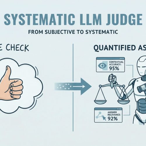
In this article, you will learn how to evaluate large language model applications using RAGAs and G-Eval-based frameworks in a practical, hands-on workflow. Topics we will cover include: How to use RAGAs to measure faithfulness and answer relevancy in retrieval-augmented systems. How to structure evaluation datasets and integrate them into a testing pipeline. How to apply G-Eval via DeepEval to assess qualitative aspects like coherence. Let’s get started. A Hands-On Guide to Testing Agents with RAGAs and G-EvalImage by Editor Introduction RAGAs (Retrieval-Augmented Generation Assessment) is an open-source evaluation framework that replaces subjective “vibe checks” with a systematic, LLM-driven “judge” to quantify the quality of RAG pipelines. It assesses a triad of desirable RAG properties, including contextual accuracy and answer relevance. RAGAs has also evolved to support not only RAG architectures but also agent-based applications, where methodologies like G-Eval play a role in defining custom, interpretable evaluation criteria. This article presents a hands-on guide to understanding how to test large language model and agent-based applications using both RAGAs and frameworks based on G-Eval. Concretely, we will leverage DeepEval, which integrates multiple evaluation metrics into a unified testing sandbox. If you are unfamiliar with evaluation frameworks like RAGAs, consider reviewing this related article first. Step-by-Step Guide This example is designed to work both in a standalone Python IDE and in a Google Colab notebook. You may need to pip install some libraries along the way to resolve potential ModuleNotFoundError issues, which occur when attempting to import modules that are not installed in your environment. We begin by defining a function that takes a user query as input and interacts with an LLM API (such as OpenAI) to generate a response. This is a simplified agent that encapsulates a basic input-response workflow. import openai def simple_agent(query): # NOTE: this is a ‘mock’ agent loop # In a real scenario, you would use a system prompt to define tool usage prompt = f”You are a helpful assistant. Answer the user query: {query}” # Example using OpenAI (this can be swapped for Gemini or another provider) response = openai.chat.completions.create( model=”gpt-3.5-turbo”, messages=[{“role”: “user”, “content”: prompt}] ) return response.choices[0].message.content import openai   def simple_agent(query):     # NOTE: this is a ‘mock’ agent loop     # In a real scenario, you would use a system prompt to define tool usage     prompt = f“You are a helpful assistant. Answer the user query: {query}”          # Example using OpenAI (this can be swapped for Gemini or another provider)     response = openai.chat.completions.create(         model=“gpt-3.5-turbo”,         messages=[{“role”: “user”, “content”: prompt}]     )     return response.choices[0].message.content In a more realistic production setting, the agent defined above would include additional capabilities such as reasoning, planning, and tool execution. However, since the focus here is on evaluation, we intentionally keep the implementation simple. Next, we introduce RAGAs. The following code demonstrates how to evaluate a question-answering scenario using the faithfulness metric, which measures how well the generated answer aligns with the provided context. from ragas import evaluate from ragas.metrics import faithfulness # Defining a simple testing dataset for a question-answering scenario data = { “question”: [“What is the capital of Japan?”], “answer”: [“Tokyo is the capital.”], “contexts”: [[“Japan is a country in Asia. Its capital is Tokyo.”]] } # Running RAGAs evaluation result = evaluate(data, metrics=[faithfulness]) from ragas import evaluate from ragas.metrics import faithfulness   # Defining a simple testing dataset for a question-answering scenario data = {     “question”: [“What is the capital of Japan?”],     “answer”: [“Tokyo is the capital.”],     “contexts”: [[“Japan is a country in Asia. Its capital is Tokyo.”]] }   # Running RAGAs evaluation result = evaluate(data, metrics=[faithfulness]) Note that you may need sufficient API quota (e.g., OpenAI or Gemini) to run these examples, which typically requires a paid account. Below is a more elaborate example that incorporates an additional metric for answer relevancy and uses a structured dataset. test_cases = [ { “question”: “How do I reset my password?”, “answer”: “Go to settings and click ‘forgot password’. An email will be sent.”, “contexts”: [“Users can reset passwords via the Settings > Security menu.”], “ground_truth”: “Navigate to Settings, then Security, and select Forgot Password.” } ] test_cases = [     {         “question”: “How do I reset my password?”,         “answer”: “Go to settings and click ‘forgot password’. An email will be sent.”,         “contexts”: [“Users can reset passwords via the Settings > Security menu.”],         “ground_truth”: “Navigate to Settings, then Security, and select Forgot Password.”     } ] Ensure that your API key is configured before proceeding. First, we demonstrate evaluation without wrapping the logic in an agent: import os from ragas import evaluate from ragas.metrics import faithfulness, answer_relevancy from datasets import Dataset # IMPORTANT: Replace “YOUR_API_KEY” with your actual API key os.environ[“OPENAI_API_KEY”] = “YOUR_API_KEY” # Convert list to Hugging Face Dataset (required by RAGAs) dataset = Dataset.from_list(test_cases) # Run evaluation ragas_results = evaluate(dataset, metrics=[faithfulness, answer_relevancy]) print(f”RAGAs Faithfulness Score: {ragas_results[‘faithfulness’]}”) import os from ragas import evaluate from ragas.metrics import faithfulness, answer_relevancy from datasets import Dataset   # IMPORTANT: Replace “YOUR_API_KEY” with your actual API key os.environ[“OPENAI_API_KEY”] = “YOUR_API_KEY”   # Convert list to Hugging Face Dataset (required by RAGAs) dataset = Dataset.from_list(test_cases)   # Run evaluation ragas_results = evaluate(dataset, metrics=[faithfulness, answer_relevancy]) print(f“RAGAs Faithfulness Score: {ragas_results[‘faithfulness’]}”) To simulate an agent-based workflow, we can encapsulate the evaluation logic into a reusable function: import os from ragas import evaluate from ragas.metrics import faithfulness, answer_relevancy from datasets import Dataset def evaluate_ragas_agent(test_cases, openai_api_key=”YOUR_API_KEY”): “””Simulates a simple AI agent that performs RAGAs evaluation.””” os.environ[“OPENAI_API_KEY”] = openai_api_key # Convert test cases into a Dataset object dataset = Dataset.from_list(test_cases) # Run evaluation ragas_results = evaluate(dataset, metrics=[faithfulness, answer_relevancy]) return ragas_results 1 2 3 4 5 6 7 8 9 10 11 12 13 14 15 16 17 import os from ragas import evaluate from ragas.metrics import faithfulness, answer_relevancy from datasets import Dataset   def evaluate_ragas_agent(test_cases, openai_api_key=“YOUR_API_KEY”):     “”“Simulates a simple AI agent that performs RAGAs evaluation.”“”          os.environ[“OPENAI_API_KEY”] = openai_api_key       # Convert test cases into a Dataset object     dataset = Dataset.from_list(test_cases)       # Run evaluation     ragas_results = evaluate(dataset,

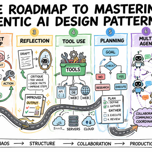
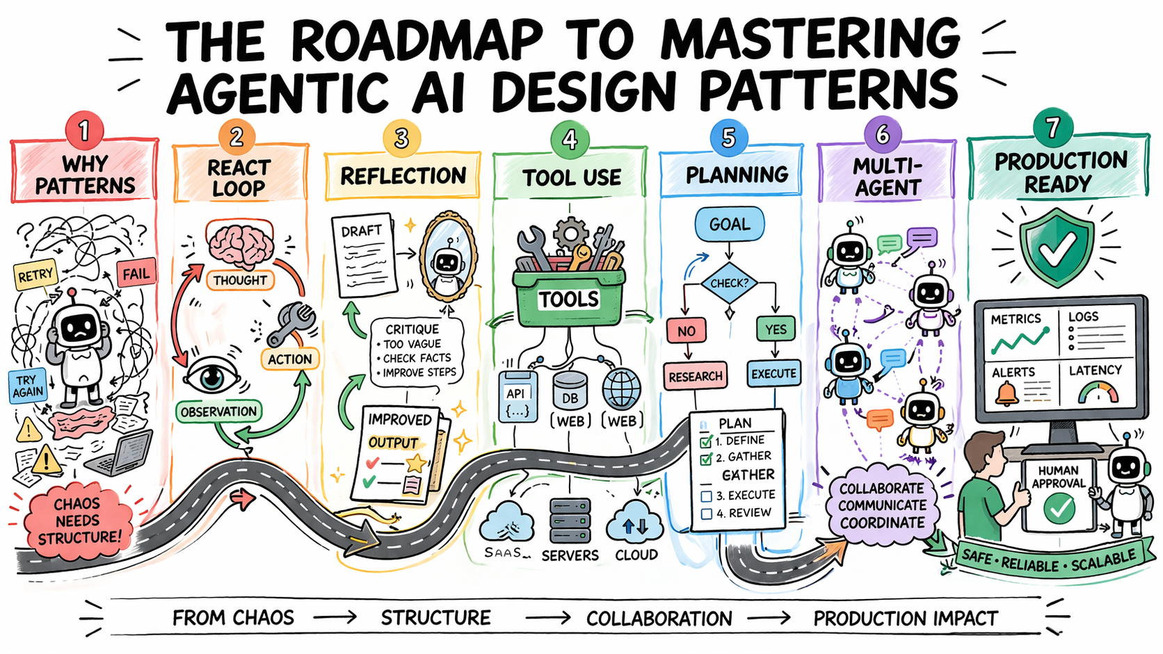
In this article, you will learn how to systematically select and apply agentic AI design patterns to build reliable, scalable agent systems. Topics we will cover include: Why design patterns are essential for predictable agent behavior Core agentic patterns such as ReAct, Reflection, Planning, and Tool Use How to evaluate, scale, and safely deploy agentic systems in production Let’s get started. The Roadmap to Mastering Agentic AI Design PatternsImage by Author Introduction Most agentic AI systems are built pattern by pattern, decision by decision, without any governing framework for how the agent should reason, act, recover from errors, or hand off work to other agents. Without structure, agent behavior is hard to predict, harder to debug, and nearly impossible to improve systematically. The problem compounds in multi-step workflows, where a bad decision early in a run affects every step that follows. Agentic design patterns are reusable approaches for recurring problems in agentic system design. They help establish how an agent reasons before acting, how it evaluates its own outputs, how it selects and calls tools, how multiple agents divide responsibility, and when a human needs to be in the loop. Choosing the right pattern for a given task is what makes agent behavior predictable, debuggable, and composable as requirements grow. This article offers a practical roadmap to understanding agentic AI design patterns. It explains why pattern selection is an architectural decision and then works through the core agentic design patterns used in production today. For each, it covers when the pattern fits, what trade-offs it carries, and how patterns layer together in real systems. Step 1: Understanding Why Design Patterns Are Necessary Before you study any specific pattern, you need to reframe what you’re actually trying to solve. The instinct for many developers is to treat agent failures as prompting failures. If the agent did the wrong thing, the fix is a better system prompt. Sometimes that is true. But more often, the failure is architectural. An agent that loops endlessly is failing because no explicit stopping condition was designed into the loop. An agent that calls tools incorrectly does not have a clear contract for when to invoke which tool. An agent that produces inconsistent outputs given identical inputs is operating without a structured decision framework. Design patterns exist to solve exactly these problems. They are repeatable architectural templates that define how an agent’s loop should behave: how it decides what to do next, when to stop, how to recover from errors, and how to interact reliably with external systems. Without them, agent behavior becomes almost impossible to debug or scale. There is also a pattern-selection problem that trips up teams early. The temptation is to reach for the most capable, most sophisticated pattern available — multi-agent systems, complex orchestration, dynamic planning. But the cost of premature complexity in agentic systems is steep. More model calls mean higher latency and token costs. More agents mean more failure surfaces. More orchestration means more coordination bugs. The expensive mistake is jumping to complex patterns before you have hit clear limitations with simpler ones. The practical implication: Treat pattern selection the way you would treat any production architecture decision. Start with the problem, not the pattern. Define what the agent needs to do, what can go wrong, and what “working correctly” looks like. Then pick the simplest pattern that handles those requirements. Further learning: AI agent design patterns | Google Cloud and Agentic AI Design Patterns Introduction and walkthrough | Amazon Web Services. Step 2: Learning the ReAct Pattern as Your Default Starting Point ReAct — Reasoning and Acting — is the most foundational agentic design pattern and the right default for most complex, unpredictable tasks. It combines chain-of-thought reasoning with external tool use in a continuous feedback loop. The structure alternates between three phases: Thought: the agent reasons about what to do next Action: the agent invokes a tool, calls an API, or runs code Observation: the agent processes the result and updates its plan This repeats until the task is complete or a stopping condition is reached. ReAct PatternImage by Author What makes the pattern effective is that it externalizes reasoning. Every decision is visible, so when the agent fails, you can see exactly where the logic broke down rather than debugging a black-box output. It also prevents premature conclusions by grounding each reasoning step in an observable result before proceeding, which reduces hallucination when models jump to answers without real-world feedback. The trade-offs are real. Each loop iteration requires an additional model call, increasing latency and cost. Incorrect tool output propagates into subsequent reasoning steps. Non-deterministic model behavior means identical inputs can produce different reasoning paths, which creates consistency problems in regulated environments. Without an explicit iteration cap, the loop can run indefinitely and costs can compound quickly. Use ReAct when the solution path is not predetermined: adaptive problem-solving, multi-source research, and customer support workflows with variable complexity. Avoid it when speed is the priority or when inputs are well-defined enough that a fixed workflow would be faster and cheaper. Further reading: ReAct: Synergizing Reasoning and Acting in Language Models and What Is a ReAct Agent? | IBM Step 3: Adding Reflection to Improve Output Quality Reflection gives an agent the ability to evaluate and revise its own outputs before they reach the user. The structure is a generation-critique-refinement cycle: the agent produces an initial output, assesses it against defined quality criteria, and uses that assessment as the basis for revision. The cycle runs for a set number of iterations or until the output meets a defined threshold. Reflection PatternImage by Author The pattern is particularly effective when critique is specialized. An agent reviewing code can focus on bugs, edge cases, or security issues. One reviewing a contract can check for missing clauses or logical inconsistencies. Connecting the critique step to external verification tools — a linter, a compiler, or a schema validator — compounds the gains further, because the agent receives deterministic feedback rather than relying solely

In this article, you will learn how to use Python’s itertools module to simplify common feature engineering tasks with clean, efficient patterns. Topics we will cover include: Generating interaction, polynomial, and cumulative features with itertools. Building lookup grids, lag windows, and grouped aggregates for structured data workflows. Using iterator-based tools to write cleaner, more composable feature engineering code. On we go. 7 Essential Python Itertools for Feature EngineeringImage by Editor Introduction Feature engineering is where most of the real work in machine learning happens. A good feature often improves a model more than switching algorithms. Yet this step usually leads to messy code with nested loops, manual indexing, hand-built combinations, and the like. Python’s itertools module is a standard library toolkit that most data scientists know exists but rarely reach for when building features. That’s a missed opportunity, as itertools is designed for working with iterators efficiently. A lot of feature engineering, at its core, is structured iteration over pairs of variables, sliding windows, grouped sequences, or every possible subset of a feature set. In this article, you’ll work through seven itertools functions that solve common feature engineering problems. We’ll spin up sample e-commerce data and cover interaction features, lag windows, category combinations, and more. By the end, you’ll have a set of patterns you can drop directly into your own feature engineering pipelines. You can get the code on GitHub. 1. Generating Interaction Features with combinations Interaction features capture the relationship between two variables — something neither variable expresses alone. Manually listing every pair from a multi-column dataset is tedious. combinations in the itertools module does it in one line. Let’s code an example to create interaction features using combinations: import itertools import pandas as pd df = pd.DataFrame({ “avg_order_value”: [142.5, 89.0, 210.3, 67.8, 185.0], “discount_rate”: [0.10, 0.25, 0.05, 0.30, 0.15], “days_since_signup”: [120, 45, 380, 12, 200], “items_per_order”: [3.2, 1.8, 5.1, 1.2, 4.0], “return_rate”: [0.05, 0.18, 0.02, 0.22, 0.08], }) numeric_cols = df.columns.tolist() for col_a, col_b in itertools.combinations(numeric_cols, 2): feature_name = f”{col_a}_x_{col_b}” df[feature_name] = df[col_a] * df[col_b] interaction_cols = [c for c in df.columns if “_x_” in c] print(df[interaction_cols].head()) 1 2 3 4 5 6 7 8 9 10 11 12 13 14 15 16 17 18 19 import itertools import pandas as pd   df = pd.DataFrame({     “avg_order_value”:    [142.5, 89.0, 210.3, 67.8, 185.0],     “discount_rate”:      [0.10,  0.25, 0.05,  0.30, 0.15],     “days_since_signup”:  [120,   45,   380,   12,   200],     “items_per_order”:    [3.2,   1.8,  5.1,   1.2,  4.0],     “return_rate”:        [0.05,  0.18, 0.02,  0.22, 0.08], })   numeric_cols = df.columns.tolist()   for col_a, col_b in itertools.combinations(numeric_cols, 2):     feature_name = f“{col_a}_x_{col_b}”     df[feature_name] = df[col_a] * df[col_b]   interaction_cols = [c for c in df.columns if “_x_” in c] print(df[interaction_cols].head()) Truncated output: avg_order_value_x_discount_rate avg_order_value_x_days_since_signup \ 0 14.250 17100.0 1 22.250 4005.0 2 10.515 79914.0 3 20.340 813.6 4 27.750 37000.0 avg_order_value_x_items_per_order avg_order_value_x_return_rate \ 0 456.00 7.125 1 160.20 16.020 2 1072.53 4.206 3 81.36 14.916 4 740.00 14.800 … days_since_signup_x_return_rate items_per_order_x_return_rate 0 6.00 0.160 1 8.10 0.324 2 7.60 0.102 3 2.64 0.264 4 16.00 0.320 1 2 3 4 5 6 7 8 9 10 11 12 13 14 15 16 17 18 19 20 21    avg_order_value_x_discount_rate  avg_order_value_x_days_since_signup  \ 0                           14.250                              17100.0   1                           22.250                               4005.0   2                           10.515                              79914.0   3                           20.340                                813.6   4                           27.750                              37000.0        avg_order_value_x_items_per_order  avg_order_value_x_return_rate  \ 0                             456.00                          7.125   1                             160.20                         16.020   2                            1072.53                          4.206   3                              81.36                         14.916   4                             740.00                         14.800   …      days_since_signup_x_return_rate  items_per_order_x_return_rate   0                             6.00                          0.160   1                             8.10                          0.324   2                             7.60                          0.102   3                             2.64                          0.264   4                            16.00                          0.320   combinations(numeric_cols, 2) generates every unique pair exactly once without duplicates. With 5 columns, that is 10 pairs; with 10 columns, it is 45. This approach scales as you add columns. 2. Building Cross-Category Feature Grids with product itertools.product gives you the Cartesian product of two or more iterables — every possible combination across them — including repeats across different groups. In the e-commerce sample we’re working with, this is useful when you want to build a feature matrix across customer segments and product categories. import itertools customer_segments = [“new”, “returning”, “vip”] product_categories = [“electronics”, “apparel”, “home_goods”, “beauty”] channels = [“mobile”, “desktop”] # All segment × category × channel combinations combos = list(itertools.product(customer_segments, product_categories, channels)) grid_df = pd.DataFrame(combos, columns=[“segment”, “category”, “channel”]) # Simulate a conversion rate lookup per combination import numpy as np np.random.seed(7) grid_df[“avg_conversion_rate”] = np.round( np.random.uniform(0.02, 0.18, size=len(grid_df)), 3 ) print(grid_df.head(12)) print(f”\nTotal combinations: {len(grid_df)}”) 1 2 3 4 5 6 7 8 9 10 11 12 13 14 15 16 17 18 19 20 import itertools   customer_segments = [“new”, “returning”, “vip”] product_categories = [“electronics”, “apparel”, “home_goods”, “beauty”] channels = [“mobile”, “desktop”]   # All segment × category × channel combinations combos = list(itertools.product(customer_segments, product_categories, channels))   grid_df = pd.DataFrame(combos, columns=[“segment”, “category”, “channel”])   # Simulate a conversion rate lookup per combination import numpy as np np.random.seed(7) grid_df[“avg_conversion_rate”] = np.round(     np.random.uniform(0.02, 0.18, size=len(grid_df)), 3 )   print(grid_df.head(12)) print(f“\nTotal combinations: {len(grid_df)}”) Output: segment category channel avg_conversion_rate 0 new electronics mobile 0.032 1 new electronics desktop 0.145 2 new apparel mobile 0.090 3 new apparel desktop 0.136 4 new home_goods mobile 0.176 5 new home_goods desktop 0.106 6 new beauty mobile 0.100 7 new beauty desktop 0.032 8 returning electronics mobile 0.063 9 returning electronics desktop 0.100 10 returning apparel mobile 0.129 11 returning apparel desktop 0.149 Total combinations: 24       segment     category  channel  avg_conversion_rate 0         new  electronics   mobile                0.032 1         new  electronics  desktop                0.145 2         new      apparel   mobile                0.090 3         new      apparel  desktop                0.136 4         new   home_goods   mobile                0.176 5         new   home_goods  desktop                0.106 6         new       beauty   mobile                0.100 7         new       beauty  desktop                0.032 8   returning  electronics   mobile                0.063 9   returning  electronics  desktop                0.100 10  returning      apparel   mobile                0.129 11  returning      apparel  desktop                0.149   Total combinations: 24 This grid can then be merged back onto your main transaction dataset as a lookup feature, as every row gets the expected conversion rate for its specific segment × category × channel bucket. product ensures you haven’t missed any valid combination when building that grid. 3. Flattening Multi-Source Feature Sets with chain In most pipelines, features come from multiple sources: a customer profile table, a product metadata table, and a browsing history table. You often need to flatten these into a single feature list for column selection

In this article, you will learn how reranking improves the relevance of results in retrieval-augmented generation (RAG) systems by going beyond what retrievers alone can achieve. Topics we will cover include: How rerankers refine retriever outputs to deliver better answers Five top reranker models to test in 2026 Final thoughts on choosing the right reranker for your system Let’s get started. Top 5 Reranking Models to Improve RAG ResultsImage by Editor Introduction If you have worked with retrieval-augmented generation (RAG) systems, you have probably seen this problem. Your retriever brings back “relevant” chunks, but many of them are not actually useful. The final answer ends up noisy, incomplete, or incorrect. This usually happens because the retriever is optimized for speed and recall, not precision. That is where reranking comes in. Reranking is the second step in a RAG pipeline. First, your retriever fetches a set of candidate chunks. Then, a reranker evaluates the query and each candidate and reorders them based on deeper relevance. In simple terms: Retriever → gets possible matches Reranker → picks the best matches This small step often makes a big difference. You get fewer irrelevant chunks in your prompt, which leads to better answers from your LLM. Benchmarks like MTEB, BEIR, and MIRACL are commonly used to evaluate these models, and most modern RAG systems rely on rerankers for production-quality results. There is no single best reranker for every use case. The right choice depends on your data, latency, cost constraints, and context length requirements. If you are starting fresh in 2026, these are the five models to test first. 1. Qwen3-Reranker-4B If I had to pick one open reranker to test first, it would be Qwen3-Reranker-4B. The model is open-sourced under Apache 2.0, supports 100+ languages, and has a 32k context length. It shows very strong published reranking results (69.76 on MTEB-R, 75.94 on CMTEB-R, 72.74 on MMTEB-R, 69.97 on MLDR, and 81.20 on MTEB-Code). It performs well across different types of data, including multiple languages, long documents, and code. 2. NVIDIA nv-rerankqa-mistral-4b-v3 For question-answering RAG over text passages, nv-rerankqa-mistral-4b-v3 is a solid, benchmark-backed choice. It delivers high ranking accuracy across evaluated datasets, with an average Recall@5 of 75.45% when paired with NV-EmbedQA-E5-v5 across NQ, HotpotQA, FiQA, and TechQA. It is commercially ready. The main limitation is context size (512 tokens per pair), so it works best with clean chunking. 3. Cohere rerank-v4.0-pro For a managed, enterprise-friendly option, rerank-v4.0-pro is designed as a quality-focused reranker with 32k context, multilingual support across 100+ languages, and support for semi-structured JSON documents. It is suitable for production data such as tickets, CRM records, tables, or metadata-rich objects. 4. jina-reranker-v3 Most rerankers score each document independently. jina-reranker-v3 uses listwise reranking, processing up to 64 documents together in a 131k-token context window, achieving 61.94 nDCG@10 on BEIR. This approach is useful for long-context RAG, multilingual search, and retrieval tasks where relative ordering matters. It is published under CC BY-NC 4.0. 5. BAAI bge-reranker-v2-m3 Not every strong reranker needs to be new. bge-reranker-v2-m3 is lightweight, multilingual, easy to deploy, and fast at inference. It is a practical baseline. If a newer model does not significantly outperform BGE, the added cost or latency may not be justified. Final Thoughts Reranking is a simple yet powerful way to improve a RAG system. A good retriever gets you close. A good reranker gets you to the right answer. In 2026, adding a reranker is essential. Here is a shortlist of recommendations: Feature Description Best open model Qwen3-Reranker-4B Best for QA pipelines NVIDIA nv-rerankqa-mistral-4b-v3 Best managed option Cohere rerank-v4.0-pro Best for long context jina-reranker-v3 Best baseline BGE-reranker-v2-m3 This selection provides a strong starting point. Your specific use case and system constraints should guide the final choice. About Kanwal Mehreen Kanwal Mehreen is an aspiring Software Developer with a keen interest in data science and applications of AI in medicine. Kanwal was selected as the Google Generation Scholar 2022 for the APAC region. Kanwal loves to share technical knowledge by writing articles on trending topics, and is passionate about improving the representation of women in tech industry.