In this article, you will learn how to build a simple semantic search engine using sentence embeddings and nearest neighbors.
Topics we will cover include:
- Understanding the limitations of keyword-based search.
- Generating text embeddings with a sentence transformer model.
- Implementing a nearest-neighbor semantic search pipeline in Python.
Let’s get started.
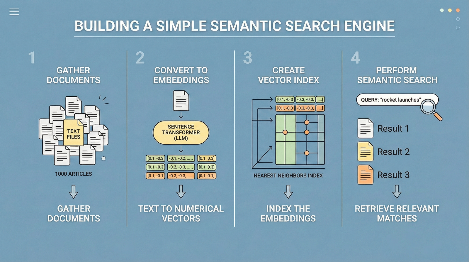
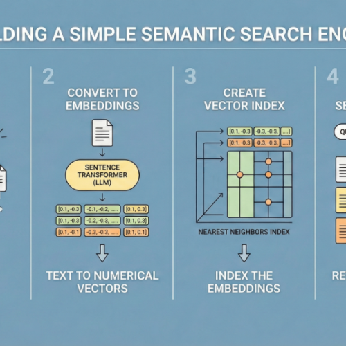
Build Semantic Search with LLM Embeddings
Image by Editor
Introduction
Traditional search engines have historically relied on keyword search. In other words, given a query like “best temples and shrines to visit in Fukuoka, Japan”, results are retrieved based on keyword matching, such that text documents containing co-occurrences of words like “temple”, “shrine”, and “Fukuoka” are deemed most relevant.
However, this classical approach is notoriously rigid, as it largely relies on exact word matches and misses other important semantic nuances such as synonyms or alternative phrasing — for example, “young dog” instead of “puppy”. As a result, highly relevant documents may be inadvertently omitted.
Semantic search addresses this limitation by focusing on meaning rather than exact wording. Large language models (LLMs) play a key role here, as some of them are trained to translate text into numerical vector representations called embeddings, which encode the semantic information behind the text. When two texts like “small dogs are very curious by nature” and “puppies are inquisitive by nature” are converted into embedding vectors, those vectors will be highly similar due to their shared meaning. Meanwhile, the embedding vectors for “puppies are inquisitive by nature” and “Dazaifu is a signature shrine in Fukuoka” will be very different, as they represent unrelated concepts.
Following this principle — which you can explore in more depth here — the remainder of this article guides you through the full process of building a compact yet efficient semantic search engine. While minimalistic, it performs effectively and serves as a starting point for understanding how modern search and retrieval systems, such as retrieval augmented generation (RAG) architectures, are built.
The code explained below can be run seamlessly in a Google Colab or Jupyter Notebook instance.
Step-by-Step Guide
First, we make the necessary imports for this practical example:
|
import pandas as pd import json from pydantic import BaseModel, Field from openai import OpenAI from google.colab import userdata from sklearn.ensemble import RandomForestClassifier from sklearn.model_selection import train_test_split from sklearn.metrics import classification_report from sklearn.preprocessing import StandardScaler |
We will use a toy public dataset called "ag_news", which contains texts from news articles. The following code loads the dataset and selects the first 1000 articles.
|
from datasets import load_dataset from sentence_transformers import SentenceTransformer from sklearn.neighbors import NearestNeighbors |
We now load the dataset and extract the "text" column, which contains the article content. Afterwards, we print a short sample from the first article to inspect the data:
|
print(“Loading dataset…”) dataset = load_dataset(“ag_news”, split=“train[:1000]”)
# Extract the text column into a Python list documents = dataset[“text”]
print(f“Loaded {len(documents)} documents.”) print(f“Sample: {documents[0][:100]}…”) |
The next step is to obtain embedding vectors (numerical representations) for our 1000 texts. As mentioned earlier, some LLMs are trained specifically to translate text into numerical vectors that capture semantic characteristics. Hugging Face sentence transformer models, such as "all-MiniLM-L6-v2", are a common choice. The following code initializes the model and encodes the batch of text documents into embeddings.
|
print(“Loading embedding model…”) model = SentenceTransformer(“all-MiniLM-L6-v2”)
# Convert text documents into numerical vector embeddings print(“Encoding documents (this may take a few seconds)…”) document_embeddings = model.encode(documents, show_progress_bar=True)
print(f“Created {document_embeddings.shape[0]} embeddings.”) |
Next, we initialize a NearestNeighbors object, which implements a nearest-neighbor strategy to find the k most similar documents to a given query. In terms of embeddings, this means identifying the closest vectors (smallest angular distance). We use the cosine metric, where more similar vectors have smaller cosine distances (and higher cosine similarity values).
|
search_engine = NearestNeighbors(n_neighbors=5, metric=“cosine”)
search_engine.fit(document_embeddings) print(“Search engine is ready!”) |
The core logic of our search engine is encapsulated in the following function. It takes a plain-text query, specifies how many top results to retrieve via top_k, computes the query embedding, and retrieves the nearest neighbors from the index.
The loop inside the function prints the top-k results ranked by similarity:
|
1 2 3 4 5 6 7 8 9 10 11 12 13 14 15 16 17 |
def semantic_search(query, top_k=3): # Embed the incoming search query query_embedding = model.encode([query])
# Retrieve the closest matches distances, indices = search_engine.kneighbors(query_embedding, n_neighbors=top_k)
print(f“\n🔍 Query: ‘{query}'”) print(“-“ * 50)
for i in range(top_k): doc_idx = indices[0][i] # Convert cosine distance to similarity (1 – distance) similarity = 1 – distances[0][i]
print(f“Result {i+1} (Similarity: {similarity:.4f})”) print(f“Text: {documents[int(doc_idx)][:150]}…\n”) |
And that’s it. To test the function, we can formulate a couple of example search queries:
|
semantic_search(“Wall street and stock market trends”) semantic_search(“Space exploration and rocket launches”) |
The results are ranked by similarity (truncated here for clarity):
|
1 2 3 4 5 6 7 8 9 10 11 12 13 14 15 16 17 18 19 20 21 22 |
🔍 Query: ‘Wall street and stock market trends’ ————————————————————————— Result 1 (Similarity: 0.6258) Text: Stocks Higher Despite Soaring Oil Prices NEW YORK – Wall Street shifted higher Monday as bargain hunters shrugged off skyrocketing oil prices and boug...
Result 2 (Similarity: 0.5586) Text: Stocks Sharply Higher on Dip in Oil Prices NEW YORK – A drop in oil prices and upbeat outlooks from Wal–Mart and Lowe‘s prompted new bargain-hunting o…
Result 3 (Similarity: 0.5459) Text: Strategies for a Sideways Market (Reuters) Reuters – The bulls and the bears are in this together, scratching their heads and wondering what’s going t...
🔍 Query: ‘Space exploration and rocket launches’ ————————————————————————— Result 1 (Similarity: 0.5803) Text: Redesigning Rockets: NASA Space Propulsion Finds a New Home (SPACE.com) SPACE.com – While the exploration of the Moon and other planets in our solar s...
Result 2 (Similarity: 0.5008) Text: Canadian Team Joins Rocket Launch Contest (AP) AP – The #36;10 million competition to send a private manned rocket into space started looking more li…
Result 3 (Similarity: 0.4724) Text: The Next Great Space Race: SpaceShipOne and Wild Fire to Go For the Gold (SPACE.com) SPACE.com – A piloted rocket ship race to claim a #36;10 million… |
Summary
What we have built here can be seen as a gateway to retrieval augmented generation systems. While this example is intentionally simple, semantic search engines like this form the foundational retrieval layer in modern architectures that combine semantic search with large language models.
Now that you know how to build a basic semantic search engine, you may want to explore retrieval augmented generation systems in more depth.