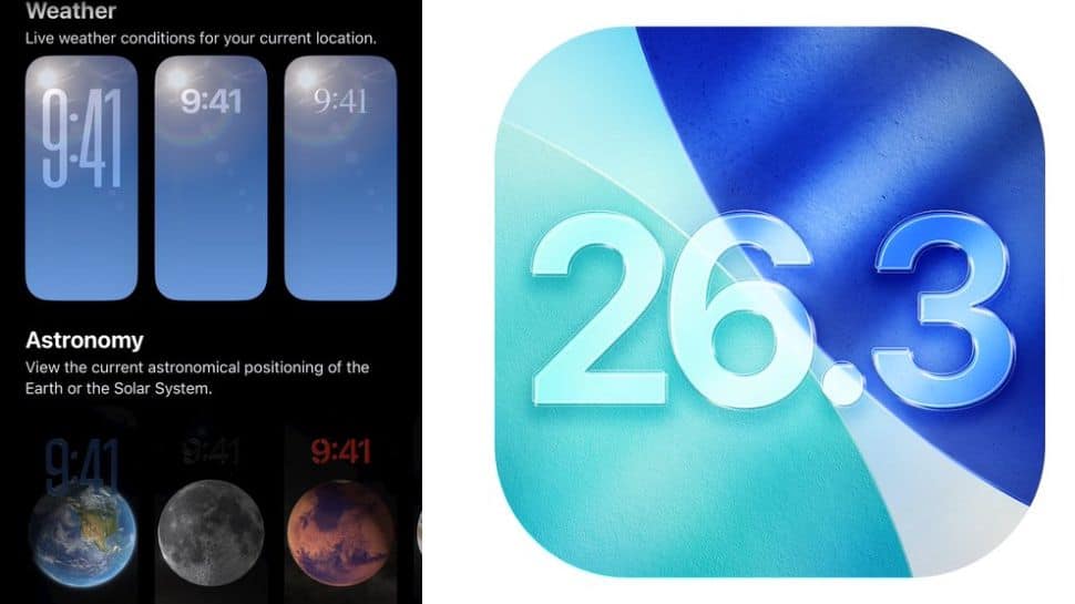
Apple iOS 26.3 Beta Update: Just days after rolling out the iOS 26.2 update, Apple has started releasing the iOS 26.3 beta 1 for eligible devices. The update is mainly aimed at developers, giving an early look at what’s coming next. While iOS 26.3 does not bring big visual changes, it focuses on how users interact with Apple’s ecosystem. However, the more new features are expected to appear in the next beta update in the new year. The stable iOS 26.3 version is likely to launch in January or February. In this Apple iOS 26.3 Beta 1 Update, one particular feature has garnered the spotlight: the Transfer to Android functionality, which makes it easier to transfer data like photos, messages, notes, passwords, and apps to an Android device. Apple iOS 26.3 Beta 1 Update: How To Move Files From iPhone To Android Add Zee News as a Preferred Source With iOS 26.3, Apple now offers a built-in tool that helps users transfer data from an iPhone to an Android phone. There is no need to install extra apps or use third-party tools. You simply keep both phones close, follow a few on-screen steps, and select what you want to move. Photos, videos, messages, notes, and basic account details can be transferred easily. However, some data will not move, such as health information, Bluetooth connections, and locked notes. These will need to be set up manually. To use this feature, both phones must be updated, and Wi-Fi and Bluetooth should be turned on. The connection is made using a QR code or a session code, depending on the Android phone. The tool works with different Android brands, not just one system. (Also Read: OpenAI Launches Faster ChatGPT Images With GPT-Image 1.5 To Compete With Gemini Nano Banana: Check Features, Availability, And How To Create Images) Apple iOS 26.3 Beta 1 Update: What’s New The update introduces a new Notification Forwarding feature that lets iPhone users send incoming notifications to third-party wearable devices, such as Android smartwatches. This option can be found in the Settings app under Notifications, where a new “Notification Forwarding” section has been added. The update also brings changes to Lock Screen customization with a separate Weather wallpaper section. Earlier, Weather and Astronomy wallpapers were grouped together, but Weather now has its own category. Apple has also added three ready-made Weather wallpapers, each with different clock fonts and weather widgets, helping users better understand how the Weather wallpaper works. 

OpenAI GPT Image Generator: In the world of fast-paced technology, the race to create the best AI image-generation models is hearing up as OpenAI has supercharged ChatGPT Images with the launch of a new model called GPT Image 1.5. The new model is designed to compete directly with Google’s Gemini Nano Banana Pro and brings several key improvements. This model is claimed to be four times faster than the previous model. According to OpenAI, the update delivers faster image generation, more accurate edits, and noticeably better image quality. Apart from this model, the company has also launched a dedicated Images space within ChatGPT, giving users access to preset filters and ready-to-use prompts for easier and quicker image creation. As mentioned by OpenAI, the upgraded model follows your instructions better and creates detailed images in lesser time as compared to its predecessor. OpenAI GPT Image 1.5: Features And Availability Add Zee News as a Preferred Source With the latest update, OpenAI has introduced a dedicated Images section in the ChatGPT sidebar, making image generation and editing easier to access. The focus this time is clearly on performance, as the Images tool not only generates visuals from text prompts but also allows users to add, combine, and even blend multiple images, similar to advanced tools like Nano Banana Pro. ChatGPT Images also offers preset prompts that users can experiment with, while still allowing room to add their own creative ideas. From the left-side Images panel, users can explore different styles, discover new visual concepts, and view their image generation history. Alongside the model upgrade, OpenAI has rolled out a new Images space across both mobile and web, featuring ready-made styles, filters, and inspiration to help users get started quickly. Adding further, users can edit images by adding or removing objects, trying out clothing, and changing styles, while the new 1.5 model improves the generation of clear and legible text within AI-created images. (Also Read: Google Translate Brings Real-Time Translation To Any Headphones: How To Use It And How It Differs From Apple’s Live Translation) How To Create Image With ChatGPT Image 1.5 Step 1: First things first, open the ChatGPT app on your smartphone or visit the official website on your computer. Step 2: Start a new chat and tap on the plus (+) icon located at the bottom-left corner of the chat box. Step 3: This will take you to a new interface where you can upload the photo you want to edit. Step 4: Once uploaded, choose any preset filter available, depending on your preference. Step 5: Alternatively, you can enter a detailed prompt describing all the changes you want in the image. Step 6: After this, wait for a few seconds while the image is processed and generated. Conclusion: Despite all the buzz around AI, image generation has clearly become the main focus for tech giants. This is evident from Google’s claim that more than 500 billion images have already been generated using Nano Banana and its Pro version. 

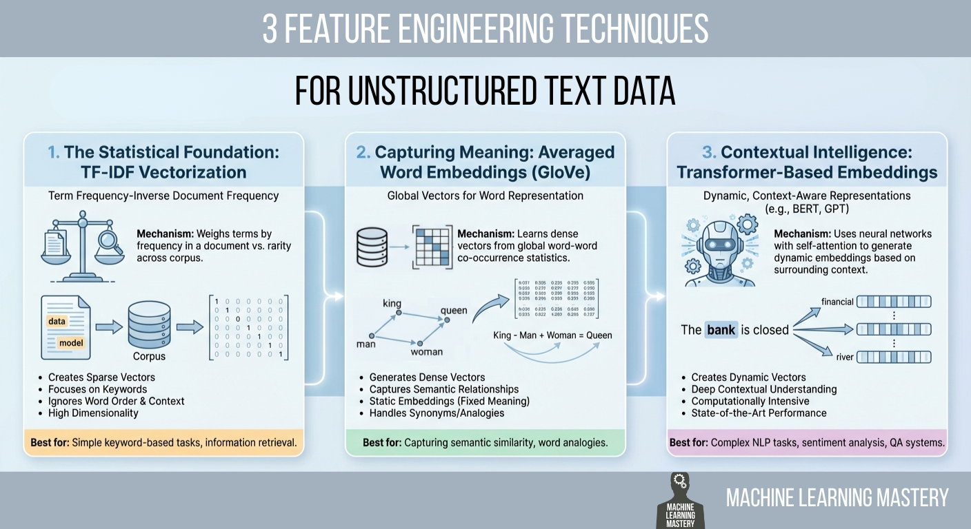
In this article, you will learn practical ways to convert raw text into numerical features that machine learning models can use, ranging from statistical counts to semantic and contextual embeddings. Topics we will cover include: Why TF-IDF remains a strong statistical baseline and how to implement it. How averaged GloVe word embeddings capture meaning beyond keywords. How transformer-based embeddings provide context-aware representations. Let’s get right into it. 3 Feature Engineering Techniques for Unstructured Text DataImage by Editor Introduction Machine learning models possess a fundamental limitation that often frustrates newcomers to natural language processing (NLP): they cannot read. If you feed a raw email, a customer review, or a legal contract into a logistic regression or a neural network, the process will fail immediately. Algorithms are mathematical functions that operate on equations, and they require numerical input to function. They do not understand words; they understand vectors. Feature engineering for text is a crucial process that bridges this gap. It is the act of translating the qualitative nuances of human language into quantitative lists of numbers that a machine can process. This translation layer is often the decisive factor in a model’s success. A sophisticated algorithm fed with poorly engineered features will perform worse than a simple algorithm fed with rich, representative features. The field has undergone significant evolution over the past few decades. It has evolved from simple counting mechanisms that treat documents as bags of unrelated words to complex deep learning architectures that understand the context of a word based on its surrounding words. This article covers three distinct approaches to this problem, ranging from the statistical foundations of TF-IDF to the semantic averaging of GloVe vectors, and finally to the state-of-the-art contextual embeddings provided by transformers. 1. The Statistical Foundation: TF-IDF Vectorization The most straightforward way to turn text into numbers is to count them. This was the standard for decades. You can simply count the number of times a word appears in a document, a technique known as bag of words. However, raw counts have a significant flaw. In almost any English text, the most frequent words are grammatically necessary but semantically empty articles and prepositions like “the,” “is,” “and,” or “of.” If you rely on raw counts, these common words will dominate your data, drowning out the rare, specific words that actually give the document its meaning. To solve this, we use term frequency–inverse document frequency (TF-IDF). This technique weighs words not just by how often they appear in a specific document, but by how rare they are across the entire dataset. It is a statistical balancing act designed to penalize common words and reward unique ones. The first part, term frequency (TF), measures how frequently a term occurs in a document. The second part, inverse document frequency (IDF), measures the importance of a term. The IDF score is calculated by taking the logarithm of the total number of documents divided by the number of documents that contain the specific term. If the word “data” appears in every single document in your dataset, its IDF score approaches zero, effectively cancelling it out. Conversely, if the word “hallucination” appears in only one document, its IDF score is very high. When you multiply TF by IDF, the result is a feature vector that highlights exactly what makes a specific document unique compared to the others. Implementation and Code Explanation We can implement this efficiently using the scikit-learn TfidfVectorizer. In this example, we take a small corpus of three sentences and convert them into a matrix of numbers. from sklearn.feature_extraction.text import TfidfVectorizer import pandas as pd # 1. Define a small corpus of text documents = [ “The quick brown fox jumps.”, “The quick brown fox runs fast.”, “The slow brown dog sleeps.” ] # 2. Initialize the Vectorizer # We limit the features to the top 100 words to keep the vector size manageable vectorizer = TfidfVectorizer(max_features=100) # 3. Fit and Transform the documents tfidf_matrix = vectorizer.fit_transform(documents) # 4. View the result as a DataFrame for clarity feature_names = vectorizer.get_feature_names_out() df_tfidf = pd.DataFrame(tfidf_matrix.toarray(), columns=feature_names) print(df_tfidf) 1 2 3 4 5 6 7 8 9 10 11 12 13 14 15 16 17 18 19 20 21 22 from sklearn.feature_extraction.text import TfidfVectorizer import pandas as pd   # 1. Define a small corpus of text documents = [     “The quick brown fox jumps.”,     “The quick brown fox runs fast.”,     “The slow brown dog sleeps.” ]   # 2. Initialize the Vectorizer # We limit the features to the top 100 words to keep the vector size manageable vectorizer = TfidfVectorizer(max_features=100)   # 3. Fit and Transform the documents tfidf_matrix = vectorizer.fit_transform(documents)   # 4. View the result as a DataFrame for clarity feature_names = vectorizer.get_feature_names_out() df_tfidf = pd.DataFrame(tfidf_matrix.toarray(), columns=feature_names)   print(df_tfidf) The code begins by importing the necessary TfidfVectorizer class. We define a list of strings that serves as our raw data. When we call fit_transform, the vectorizer first learns the vocabulary of the entire list (the “fit” step) and then transforms each document into a vector based on that vocabulary.   The output is a Pandas DataFrame, where each row represents a sentence, and each column represents a unique word found in the data. 2. Capturing Meaning: Averaged Word Embeddings (GloVe) While TF-IDF is powerful for keyword matching, it suffers from a lack of semantic understanding. It treats the words “good” and “excellent” as completely unrelated mathematical features because they have different spellings. It does not know that they mean nearly the same thing. To solve this, we move to word embeddings. Word embeddings are a technique where words are mapped to vectors of real numbers. The core idea is that words with similar meanings should have similar mathematical representations. In this vector space, the distance between the vector for “king” and “queen” is roughly similar to the distance between “man” and “woman.” One of the most popular pre-trained embedding sets is GloVe (global vectors for word representation), developed by researchers at

Large Language Models (LLMs) can produce varied, creative, and sometimes surprising outputs even when given the same prompt. This randomness is not a bug but a core feature of how the model samples its next token from a probability distribution. In this article, we break down the key sampling strategies and demonstrate how parameters such as temperature, top-k, and top-p influence the balance between consistency and creativity. In this tutorial, we take a hands-on approach to understand: How logits become probabilities How temperature, top-k, and top-p sampling work How different sampling strategies shape the model’s next-token distribution By the end, you will understand the mechanics behind LLM inference and be able to adjust the creativity or determinism of the output. Let’s get started. How LLMs Choose Their Words: A Practical Walk-Through of Logits, Softmax and SamplingPhoto by Colton Duke. Some rights reserved. Overview This article is divided into four parts; they are: How Logits Become Probabilities Temperature Top-k Sampling Top-p Sampling How Logits Become Probabilities When you ask an LLM a question, it outputs a vector of logits. Logits are raw scores the model assigns to each possible next token in its vocabulary. If the model has a vocabulary of $V$ tokens, it will output a vector of $V$ logits for each next word position. A logit is a real number. It is converted into a probability by the softmax function: $$p_i = \frac{e^{x_i}}{\sum_{j=1}^{V} e^{x_j}}$$ where $x_i$ is the logit for token $i$ and $p_i$ is the corresponding probability. Softmax transforms these raw scores into a probability distribution. All $p_i$ are positive, and their sum is 1. Suppose we give the model this prompt: Today’s weather is so ___ The model considers every token in its vocabulary as a possible next word. For simplicity, let’s say there are only 6 tokens in the vocabulary: wonderful cloudy nice hot gloomy delicious wonderful cloudy nice hot gloomy delicious The model produces one logit for each token. Here’s an example set of logits the model might output and the corresponding probabilities based on the softmax function: Token Logit Probability wonderful 1.2 0.0457 cloudy 2.0 0.1017 nice 3.5 0.4556 hot 3.0 0.2764 gloomy 1.8 0.0832 delicious 1.0 0.0374 You can confirm this by using the softmax function from PyTorch: import torch import torch.nn.functional as F vocab = [“wonderful”, “cloudy”, “nice”, “hot”, “gloomy”, “delicious”] logits = torch.tensor([1.2, 2.0, 3.5, 3.0, 1.8, 1.0]) probs = F.softmax(logits, dim=-1) print(probs) # Output: # tensor([0.0457, 0.1017, 0.4556, 0.2764, 0.0832, 0.0374]) import torch import torch.nn.functional as F   vocab = [“wonderful”, “cloudy”, “nice”, “hot”, “gloomy”, “delicious”] logits = torch.tensor([1.2, 2.0, 3.5, 3.0, 1.8, 1.0]) probs = F.softmax(logits, dim=–1) print(probs) # Output: # tensor([0.0457, 0.1017, 0.4556, 0.2764, 0.0832, 0.0374]) Based on this result, the token with the highest probability is “nice”. LLMs don’t always select the token with the highest probability; instead, they sample from the probability distribution to produce a different output each time. In this case, there’s a 46% probability of seeing “nice”. If you want the model to give a more creative answer, how can you change the probability distribution such that “cloudy”, “hot”, and other answers would also appear more often? Temperature Temperature ($T$) is a model inference parameter. It is not a model parameter; it is a parameter of the algorithm that generates the output. It scales logits before applying softmax: $$p_i = \frac{e^{x_i / T}}{\sum_{j=1}^{V} e^{x_j / T}}$$ You can expect the probability distribution to be more deterministic if $T<1$, since the difference between each value of $x_i$ will be exaggerated. On the other hand, it will be more random if $T>1$, as the difference between each value of $x_i$ will be reduced. Now, let’s visualize this effect of temperature on the probability distribution: import matplotlib.pyplot as plt import torch import torch.nn.functional as F vocab = [“wonderful”, “cloudy”, “nice”, “hot”, “gloomy”, “delicious”] logits = torch.tensor([1.2, 2.0, 3.5, 3.0, 1.8, 1.0]) # (vocab_size,) scores = logits.unsqueeze(0) # (1, vocab_size) temperatures = [0.1, 0.5, 1.0, 3.0, 10.0] fig, ax = plt.subplots(figsize=(10, 6)) for temp in temperatures: # Apply temperature scaling scores_processed = scores / temp # Convert to probabilities probs = F.softmax(scores_processed, dim=-1)[0] # Sample from the distribution sampled_idx = torch.multinomial(probs, num_samples=1).item() print(f”Temperature = {temp}, sampled: {vocab[sampled_idx]}”) # Plot the probability distribution ax.plot(vocab, probs.numpy(), marker=”o”, label=f”T={temp}”) ax.set_title(“Effect of Temperature”) ax.set_ylabel(“Probability”) ax.legend() plt.show() 1 2 3 4 5 6 7 8 9 10 11 12 13 14 15 16 17 18 19 20 21 22 23 24 25 import matplotlib.pyplot as plt import torch import torch.nn.functional as F   vocab = [“wonderful”, “cloudy”, “nice”, “hot”, “gloomy”, “delicious”] logits = torch.tensor([1.2, 2.0, 3.5, 3.0, 1.8, 1.0]) # (vocab_size,) scores = logits.unsqueeze(0) # (1, vocab_size) temperatures = [0.1, 0.5, 1.0, 3.0, 10.0]   fig, ax = plt.subplots(figsize=(10, 6)) for temp in temperatures:     # Apply temperature scaling     scores_processed = scores / temp     # Convert to probabilities     probs = F.softmax(scores_processed, dim=–1)[0]     # Sample from the distribution     sampled_idx = torch.multinomial(probs, num_samples=1).item()     print(f“Temperature = {temp}, sampled: {vocab[sampled_idx]}”)     # Plot the probability distribution     ax.plot(vocab, probs.numpy(), marker=‘o’, label=f“T={temp}”)   ax.set_title(“Effect of Temperature”) ax.set_ylabel(“Probability”) ax.legend() plt.show() This code generates a probability distribution over each token in the vocabulary. Then it samples a token based on the probability. Running this code may produce the following output: Temperature = 0.1, sampled: nice Temperature = 0.5, sampled: nice Temperature = 1.0, sampled: nice Temperature = 3.0, sampled: wonderful Temperature = 10.0, sampled: delicious Temperature = 0.1, sampled: nice Temperature = 0.5, sampled: nice Temperature = 1.0, sampled: nice Temperature = 3.0, sampled: wonderful Temperature = 10.0, sampled: delicious and the following plot showing the probability distribution for each temperature: The effect of temperature to the resulting probability distribution The model may produce the nonsensical output “Today’s weather is so delicious” if you set the temperature to 10! Top-k Sampling The model’s output is a vector of logits for each position in the output sequence. The inference algorithm converts the logits to actual words, or in LLM terms, tokens. The simplest method for selecting the next token is greedy sampling,

In this article, you will learn how to build, train, and compare an LSTM and a transformer for next-day univariate time series forecasting on real public transit data. Topics we will cover include: Structuring and windowing a time series for supervised learning. Implementing compact LSTM and transformer architectures in PyTorch. Evaluating and comparing models with MAE and RMSE on held-out data. All right, full steam ahead. Transformer vs LSTM for Time Series: Which Works Better?Image by Editor Introduction From daily weather measurements or traffic sensor readings to stock prices, time series data are present nearly everywhere. When these time series datasets become more challenging, models with a higher level of sophistication — such as ensemble methods or even deep learning architectures — can be a more convenient option than classical time series analysis and forecasting techniques. The objective of this article is to showcase how two deep learning architectures are trained and used to handle time series data — long short term memory (LSTM) and the transformer. The main focus is not merely leveraging the models, but understanding their differences when handling time series and whether one architecture clearly outperforms the other. Basic knowledge of Python and machine learning essentials is recommended. Problem Setup and Preparation For this illustrative comparison, we will consider a forecasting task on a univariate time series: given the temporally ordered previous N time steps, predict the (N+1)th value. In particular, we will use a publicly available version of the Chicago rides dataset, which contains daily recordings for bus and rail passengers in the Chicago public transit network dating back to 2001. This initial piece of code imports the libraries and modules needed and loads the dataset. We will import pandas, NumPy, Matplotlib, and PyTorch — all for the heavy lifting — along with the scikit-learn metrics that we will rely on for evaluation. import pandas as pd import numpy as np import matplotlib.pyplot as plt import torch import torch.nn as nn from sklearn.metrics import mean_squared_error, mean_absolute_error url = “https://data.cityofchicago.org/api/views/6iiy-9s97/rows.csv?accessType=DOWNLOAD” df = pd.read_csv(url, parse_dates=[“service_date”]) print(df.head()) import pandas as pd import numpy as np import matplotlib.pyplot as plt   import torch import torch.nn as nn from sklearn.metrics import mean_squared_error, mean_absolute_error   url = “https://data.cityofchicago.org/api/views/6iiy-9s97/rows.csv?accessType=DOWNLOAD” df = pd.read_csv(url, parse_dates=[“service_date”]) print(df.head()) Since the dataset contains post-COVID real data about passenger numbers — which may severely mislead the predictive power of our models due to being very differently distributed than pre-COVID data — we will filter out records from January 1, 2020 onwards. df_filtered = df[df[‘service_date’] <= ‘2019-12-31’] print(“Filtered DataFrame head:”) display(df_filtered.head()) print(“\nShape of the filtered DataFrame:”, df_filtered.shape) df = df_filtered df_filtered = df[df[‘service_date’] <= ‘2019-12-31’]   print(“Filtered DataFrame head:”) display(df_filtered.head())   print(“\nShape of the filtered DataFrame:”, df_filtered.shape) df = df_filtered A simple plot will do the job to show what the filtered data looks like: df.sort_values(“service_date”, inplace=True) ts = df.set_index(“service_date”)[“total_rides”].fillna(0) plt.plot(ts) plt.title(“CTA Daily Total Rides”) plt.show() df.sort_values(“service_date”, inplace=True) ts = df.set_index(“service_date”)[“total_rides”].fillna(0)   plt.plot(ts) plt.title(“CTA Daily Total Rides”) plt.show() Chicago rides time series dataset plotted Next, we split the time series data into training and test sets. Importantly, in time series forecasting tasks — unlike classification and regression — this partition cannot be done at random, but in a purely sequential fashion. In other words, all training instances come chronologically first, followed by test instances. This code takes the first 80% of the time series as a training set, and the remaining 20% for testing. n = len(ts) train = ts[:int(0.8*n)] test = ts[int(0.8*n):] train_vals = train.values.astype(float) test_vals = test.values.astype(float) n = len(ts) train = ts[:int(0.8*n)] test = ts[int(0.8*n):]   train_vals = train.values.astype(float) test_vals = test.values.astype(float) Furthermore, raw time series must be converted into labeled sequences (x, y) spanning a fixed time window to properly train neural network-based models upon them. For example, if we use a time window of N=30 days, the first instance will span the first 30 days of the time series, and the associated label to predict will be the 31st day, and so on. This gives the dataset an appropriate labeled format for supervised learning tasks without losing its important temporal meaning: def create_sequences(data, seq_len=30): X, y = [], [] for i in range(len(data)-seq_len): X.append(data[i:i+seq_len]) y.append(data[i+seq_len]) return np.array(X), np.array(y) SEQ_LEN = 30 X_train, y_train = create_sequences(train_vals, SEQ_LEN) X_test, y_test = create_sequences(test_vals, SEQ_LEN) # Convert our formatted data into PyTorch tensors X_train = torch.tensor(X_train).float().unsqueeze(-1) y_train = torch.tensor(y_train).float().unsqueeze(-1) X_test = torch.tensor(X_test).float().unsqueeze(-1) y_test = torch.tensor(y_test).float().unsqueeze(-1) def create_sequences(data, seq_len=30):     X, y = [], []     for i in range(len(data)–seq_len):         X.append(data[i:i+seq_len])         y.append(data[i+seq_len])     return np.array(X), np.array(y)   SEQ_LEN = 30 X_train, y_train = create_sequences(train_vals, SEQ_LEN) X_test, y_test = create_sequences(test_vals, SEQ_LEN)   # Convert our formatted data into PyTorch tensors X_train = torch.tensor(X_train).float().unsqueeze(–1) y_train = torch.tensor(y_train).float().unsqueeze(–1) X_test = torch.tensor(X_test).float().unsqueeze(–1) y_test = torch.tensor(y_test).float().unsqueeze(–1) We are now ready to train, evaluate, and compare our LSTM and transformer models! Model Training We will use the PyTorch library for the modeling stage, as it provides the necessary classes to define both recurrent LSTM layers and encoder-only transformer layers suitable for predictive tasks. First up, we have an LSTM-based RNN architecture like this: class LSTMModel(nn.Module): def __init__(self, hidden=32): super().__init__() self.lstm = nn.LSTM(1, hidden, batch_first=True) self.fc = nn.Linear(hidden, 1) def forward(self, x): out, _ = self.lstm(x) return self.fc(out[:, -1]) lstm_model = LSTMModel() class LSTMModel(nn.Module):     def __init__(self, hidden=32):         super().__init__()         self.lstm = nn.LSTM(1, hidden, batch_first=True)         self.fc = nn.Linear(hidden, 1)       def forward(self, x):         out, _ = self.lstm(x)         return self.fc(out[:, –1])   lstm_model = LSTMModel() As for the encoder-only transformer for next-day time series forecasting, we have: class SimpleTransformer(nn.Module): def __init__(self, d_model=32, nhead=4): super().__init__() self.embed = nn.Linear(1, d_model) enc_layer = nn.TransformerEncoderLayer(d_model=d_model, nhead=nhead, batch_first=True) self.transformer = nn.TransformerEncoder(enc_layer, num_layers=1) self.fc = nn.Linear(d_model, 1) def forward(self, x): x = self.embed(x) x = self.transformer(x) return self.fc(x[:, -1]) transformer_model = SimpleTransformer() class SimpleTransformer(nn.Module):     def __init__(self, d_model=32, nhead=4):         super().__init__()         self.embed = nn.Linear(1, d_model)         enc_layer = nn.TransformerEncoderLayer(d_model=d_model, nhead=nhead, batch_first=True)         self.transformer = nn.TransformerEncoder(enc_layer, num_layers=1)         self.fc = nn.Linear(d_model, 1)       def forward(self, x):         x = self.embed(x)         x = self.transformer(x)         return self.fc(x[:, –1])   transformer_model = SimpleTransformer() Note that

Oppo Reno 15C Price: Chinese brand Oppo has expanded its Reno smartphone lineup with the launch of the Oppo Reno 15C in China. However, the newly-launched smartphone could arrive in India as Oppo Reno 15. The Oppo Reno 15C has IP66 + IP68 + IP69 ratings for dust and water resistance and has 360° drop protection. The device comes in College Blue, Aurora Blue, and Starlight Bow colour option. The dual SIM (Nano+Nano) Oppo Reno 15c runs on Android 16-based ColorOS 16. Notably, the Chinese variant offers a clear indication of what Indian consumers can expect from the upcoming Reno series smartphone. Oppo Reno 15C Specifications Add Zee News as a Preferred Source The smartphone features a 6.59-inch 1.5K flat OLED display with a resolution of 2760×1256 pixels, a smooth 120Hz refresh rate, and up to 1,200 nits peak brightness. It is powered by the Snapdragon 7 Gen 4 chipset paired with an Adreno 722 GPU, offering up to 12GB of LPDDR5x RAM and up to 512GB of UFS 3.1 onboard storage. On the photography front, the handset sports a triple rear camera setup comprising a 50-megapixel wide-angle sensor with OIS, a 50-megapixel telephoto camera with OIS, and an 8-megapixel ultra-wide-angle lens, while the front houses a 50-megapixel selfie camera. (Also Read: Google Pixel 10 Pro Gets Huge Discount On THIS Platform Under Rs 1,00,000; Check Camera, Display, Battery, Price And Other Specs) The Oppo Reno 15c packs a large 6,500mAh battery with support for 80W wired fast charging. It measures 158×74.83×7.77mm and weighs around 197g. On the connectivity front, the smartphone supports Wi-Fi 6, Bluetooth, NFC, USB Type-C, and multiple navigation systems such as BeiDou, GPS, GLONASS, Galileo, and QZSS. The phone is also equipped with several sensors, including a proximity sensor, ambient light sensor, electronic compass, accelerometer, gyroscope, infrared remote control, and an in-display ultrasonic fingerprint sensor for secure authentication. Oppo Reno 15C Price The smartphone is priced starting at CNY 2,899 (approximately Rs. 37,000) for the 12GB RAM and 256GB storage variant, while the 12GB RAM and 512GB storage model carries a price tag of CNY 3,199 (around Rs. 41,000). 

New Delhi: Around 74 per cent of corporate leaders in India ranked artificial intelligence (AI) among their top three technology adoption choices, a report said on Tuesday. The report from Standard Chartered bank said that AI was followed by cloud computing at 64 per cent and digital assets at 46 per cent as next top choices. On a global scale, approximately seven in 10 corporate leaders are focusing on building strong foundational systems of emerging technologies in the short to medium term — notably cloud computing. Respondents cited AI (55 per cent) and digital assets (50 per cent) among the top three drivers shaping the future of trade digitalisation, reflecting a pragmatic view that robust underlying infrastructure must precede emerging technologies to deliver value at scale. “By prioritising connected data flows, compliance, and consistency, corporates are setting the stage for technologies like artificial intelligence and digital assets to scale responsibly and efficiently. When these underlying layers are strong, innovation can accelerate and sustain long-term growth across global value chains,” said Michael Spiegel, Global Head, Transaction Banking, Standard Chartered. Add Zee News as a Preferred Source The report said that bullish sentiment about AI is supported by government initiatives, such as the National Strategy for Artificial Intelligence. Several AI firms have been investing and expanding their operations in the world’s most populous market, the report noted. The bank said that 68 per cent of Indian respondents reported outsourcing digitalisation work completely, 30 per cent work with third‑party providers, and 3 per cent handle it entirely in‑house. Over half of the corporates cited lack of interoperability and integration as the main challenge to trade digitalisation, with regulatory and implementation challenges keeping many processes paper‑based. The report, based on a survey of 1,200 C‑suite and senior leaders across 17 markets, said that 80 per cent of respondents used banking partners to advise on digitalisation and the adoption of digital assets.

Google Translate In Real Time App: In a country like India, every journey is a conversation in itself, one that shifts languages with every mile. From a chai-side chat in a small town to a boardroom discussion in a bustling metro, words often change faster than people can keep up. That is where Google Translate quietly steps in, turning confusion into clarity. Whether you are travelling across states, attending meetings, or connecting with someone from a different culture, language barriers no longer have to slow you down. Now, Google is taking this experience a step further by offering real-time translation through the Translate app, powered by Gemini and seamlessly accessible across all headphones, making communication feel natural, instant, smooth, and effortless. More interesting part is that you do not need costly smart earbuds or special translation devices. Any regular wired or wireless headphones will do the job. If you are wondering how to use Google Translate for real-time translations on any headphones, this article will guide you step by step. Add Zee News as a Preferred Source How To Use Google Translate On Any Headphones In Real Time Step 1: Open the Google Translate app on your smartphone. Step 2: At the top, select your spoken language on the left and the language you want to understand on the right. Step 3: Tap the Conversation option located at the bottom left of the main screen. Step 4: When the prompt appears, tap the Start button to begin real-time translation. Step 5: Keep your phone close to the person who is speaking and ask them to speak clearly at a normal pace. Step 6: The app will listen through your phone’s microphone, and the translated audio will automatically play in your connected headphones. Google Translate Vs Apple Live Translation: What Makes Google’s Real-Time App Different Google’s real-time translation keeps things simple and easy to use. You do not need to buy special devices or costly earbuds. An Android phone, the Google Translate app, and any headphones, wired or wireless, are enough. Once you turn it on, you just listen while the other person speaks, and the translated voice plays in your headphones. The feature supports more than 70 languages in beta and even keeps the speaker’s voice style and pauses, so it feels natural. (Also Read: Google Pixel 10 Pro Gets Huge Discount On THIS Platform Under Rs 1,00,000; Check Camera, Display, Battery, Price And Other Specs) On the other hand, Apple takes a different path with Live Translation. It is deeply tied to the Apple ecosystem and works only with certain AirPods and an iPhone running the latest iOS with Apple Intelligence. The big advantage is two-way conversation, where both people can talk and hear translations. Apple also offers text transcripts and replay options, making it helpful but limited to Apple devices. Conclusion: Since this is a beta feature, you may notice a few bugs or minor translation errors, which are common with AI tools. Tech giant Google is actively improving the feature to make it more accurate and reliable. iPhone users are expected to get access sometime in 2026, along with a wider rollout to more countries. It is important to note that Google Translate does not work in offline mode, so you must ensure a stable network connection while using the app. 

New Delhi: In a bid to support India’s research ecosystem, Google.org, the philanthropic arm of Google, on Tuesday announced a funding of $8 million for four AI Centres of Excellence for health, agriculture, education, and sustainable cities. The centres were established by the Government, aligning with the vision to “Make AI in India and Make AI work for India”. The centres include TANUH at IISc Bangalore, which will focus on developing scalable AI solutions for effective treatment of non-communicable diseases; Airawat Research Foundation at IIT Kanpur, which will focus on pioneering research on AI to transform urban governance. The AI Centre of Excellence for Education at IIT Madras will focus on developing solutions to enhance learning and teaching outcomes, while ANNAM.AI at IIT Ropar will focus on developing data-driven solutions for agriculture and farmer welfare. Add Zee News as a Preferred Source In addition, Google announced a $2 million founding contribution to establish the new Indic Language Technologies Research Hub at IIT Bombay. The hub, set up in memory of Professor Pushpak Bhattacharyya, a pioneer in Indic language technologies and a Visiting Researcher at Google DeepMind, will aim to ensure that global AI advancements serve India’s linguistic diversity. “India is approaching artificial intelligence as a strategic national capability, not as a short-term technology trend. The four AI Centres of Excellence have been conceived as a coordinated national research mission, advancing foundational research, responsible AI, and applied solutions that serve public purpose, and contributing to our larger aspiration of Viksit Bharat 2047,” said Dharmendra Pradhan, Minister of Education. “Building a globally competitive AI ecosystem requires not only public investment, but also strong institutional leadership and long-term partnerships with industry. This effort is supported by Google and Google.org through their $8 million contribution to the AI Centres of Excellence and a $2 million founding contribution to the Indic Language Technologies Research Hub at IIT Bombay,” he added. At Google’s “Lab to Impact” dialogue, supported by the India AI Impact Summit 2026, the company also committed $400,000 to support the development of India’s Health Foundation model using Google’s MedGemma — the specialised AI model designed for healthcare. As a first step, Ajna Lens will work with experts from the All India Institute of Medical Sciences (AIIMS) to build models that will support India-specific use cases in Dermatology and OPD Triaging. The resulting models will contribute to India’s Digital Public Infrastructure, and their outcomes will be made accessible to the ecosystem. Google is also working with India’s National Health Authority (NHA) to deploy its advanced AI to convert millions of fragmented, unstructured medical records, such as doctors’ clinical and progress notes, into the international, machine-readable FHIR standard. “From foundational research to ecosystem deployment to scaled impact, our full-stack approach is equipping the country to lead a global AI-powered future, with innovations from India’s labs benefiting billions across the world,” said Dr Manish Gupta, Senior Research Director, Google DeepMind.

Google Pixel 10 Pro Discount Price In India: As we head towards 2026, there are many smartphones in the market that are available at heavy discounts. Google launched the Pixel 10 series in both the Indian and global markets. At present, the Google Pixel 10 Pro (16GB RAM+256GB storage variant), one of the best phones in the lineup, is available at a big discount on Amazon India. Notably, The smartphone is based on the Android 16 operating system with up to 7 major Android upgrades promised by Google. As we all know, the Google Pixel 10 Pro rarely waits for the spotlight; it creates its own. Known for its clean Android experience, powerful camera performance, and smart AI features, the flagship phone has always been priced at a premium. But this time, the story takes an unexpected turn. What was once a dream smartphone for many people is now easier to buy because of a major discount on the e commerce giant Amazon. Many users admired this phone earlier but could not afford it. Add Zee News as a Preferred Source Some users loved it for its camera and stylish design, while others liked its fast performance and special Pixel features. Now, the lower price makes the deal even better. The Google Pixel 10 Pro is not just about new and smart features anymore; it is also about perfect timing. If you are planning to buy a new phone, this could be the right time to upgrade. Google Pixel 10 Pro Discount: Price Breakup The smartphone is currently available on Amazon India for Rs 97,890, down from its original price of Rs 1,09,999. Customers using an Amazon Pay ICICI credit card can get up to Rs 3,000 as Amazon Pay Balance cashback, bringing the effective price to around Rs 94,890. Adding further, buyers can avail of a flat Rs 1,000 instant discount on Axis Bank credit card transactions, with a minimum purchase value of Rs 65,990. Google Pixel 10 Pro Specifications The device is powered by the Google Tensor G5 chipset, built on an advanced 3nm process and paired with a PowerVR DXT-48-1536 GPU for smooth performance and efficient graphics handling. It sports a 6.3-inch LTPO OLED display that supports a 120Hz refresh rate and delivers up to 3,300 nits of peak brightness for excellent visibility even in bright conditions. (Also Read: Redmi Note 15 5G Likely To Launch In India In New Year; Check Expected Camera, Display, Battery, Price And Other Specs) On the photography front, the smartphone comes with a versatile triple rear camera setup, featuring a 50MP primary sensor with Optical Image Stabilisation (OIS), a 48MP periscope telephoto lens offering 5x optical zoom, and a 48MP ultra-wide camera. For selfies and video calls, it is equipped with a high-resolution 42MP front camera. The smartphone is powered by a 4,870mAh battery, supported by 30W wired fast charging.